We present a comprehensive analysis of the profitability of technical trading strategies that were successful within the sample period for the cryptocurrency pairs BTC/USDT and ETH/USDT. The study covers the time period from August 2017 to October 2023 and employs rigorous data snooping tests including reality checks and stepwise tests. This approach ensures that any positive results obtained are not merely coincidental, but instead reflect the intrinsic value of the method. Our results indicate that the previously profitable technical approaches, observed prior to December 2021, generally failed to generate profits during the subsequent out-of-sample period, especially after adjusting for potential data snooping. Based on the results, it is recommended to exercise caution when relying solely on historically profitable trading strategies and advisable for investors and practitioners to validate the performance of such strategies in real-time market conditions before implementing them. The findings of the study highlight the difficulty of identifying profitable technical trading strategies in an out-of-sample context when only data from the in-sample period are available, which lends support to the efficient market hypothesis within the cryptocurrency market.
Technical analysis, also known as chartist analysis, encompasses a range of techniques utilized to generate trading recommendations for financial assets. These recommendations are derived through the analysis of historical time series data for the price of the asset, using either graphical or mathematical methods. Despite their lack of foundation in underlying fundamentals, technical analysis is extensively employed by financial practitioners across different markets. Numerous studies have confirmed the effectiveness of trading strategies based on technical indicators. For instance, Tam and Cuong 1 confirmed the effectiveness of the three most popular technical indicators in investment strategies for the Vietnam stock market. Moreover, a study conducted on technical trading rules for the NYSE index from 1962 to 1996 demonstrates their potential for profitability (Kwon and Kish 2). In addition, Ratner and Leal 3 examined the profit potential of variable length moving average trading rules in emerging equity markets. These findings underscore the practical significance of technical analysis in various financial contexts. Consequently, technical analysis serves as a valuable tool for financial practitioners seeking to generate trading recommendations for diverse financial assets.
In recent years, the cryptocurrency market has received significant attention from researchers who have explored various aspects of this market. One noteworthy study by Resta, Pagnottoni, and De Giuli 4 reveals that the implementation of technical trading rules can lead to profitable outcomes for Bitcoin. Furthermore, recent findings indicate the presence of a bi-directional causal relationship between cryptocurrency returns and volume. This discovery has important implications for both technical analysis and trend-following strategies, as emphasized by Fousekis and Tzaferi 5. In order to provide a comprehensive overview of research on cryptocurrency trading and its potential, Fang et al. 6 conducted an extensive survey in the field. Considering the existing literature, there is a growing interest in understanding the driving forces behind the cryptocurrency market. This interest encompasses a comprehensive grasp of economic fundamentals as well as behavioral considerations. By adopting this holistic perspective, researchers aim to shed light on the intricate dynamics of this emerging market.
Notwithstanding, despite previous investigations, there is still a need for a comprehensive and current examination of technical analysis in this specific market. Most existing research on this subject has limitations such as short sample timeframes, a narrow range of technical trading rules, simple performance measures, and basic analysis methods which may potentially lead to data-snooping bias.{1} Therefore, it is crucial to conduct a large-scale inquiry with a proper empirical framework to address the intriguing question of whether technical analysis can outperform the specific market.
In this paper, our objective is to investigate the practical profitability of various technical trading tactics in the cryptocurrency market. To achieve this, we utilize a comprehensive approach that combines out-of-sample performance measurements and vigilance assessment.
To commence our analysis, we divide the entire study period, including August 2017 to October 2023, into two distinct intervals: an initial in-sample period and a subsequent out-of-sample period. The in-sample period covers the time preceding December 2021, during which we evaluate the persistence of the profitability of technical trading tactics. This assessment creates a foundation for our subsequent analysis in the out-of-sample period, which starts after December 2021. Additionally, to mitigate potential concerns related to data-snooping bias, we adhere to established practices outlined in existing literature. Specifically, we draw upon the work of Neely et al. 7 and other relevant studies to employ vigilance assessment and stepwise examinations. By incorporating these methodologies in our analyses, we can correct for any predisposition towards data-snooping and ensure the unbiased and robust nature of our findings.
Through the implementation of this comprehensive approach and consideration of a wide range of technical trading strategies, we evaluate the feasibility of technical trading in the out-of-sample period using a range of assessments. We find that, depending on the time intervals, nearly all of the top-performing techniques identified in the in-sample period do not yield profits in the out-of-sample period. These findings indicate the challenges faced by traders when utilizing technical trading methods. It becomes difficult to consistently apply the same strategies over time, as even the most successful tactic identified in the in-sample period cannot consistently generate profits in the out-of-sample period.
Additionally, in conjunction with our contribution to the existing literature on the profitability of technical trading in the cryptocurrency market, specifically focusing on the BTC/USDT and ETH/USDT cryptocurrency pairs, we provide evidence that traders face significant challenges in selecting a profitable technical trading approach that can consistently succeed in subsequent out-of-sample periods. Our study’s findings demonstrate that technical trading strategies that are profitable during the in-sample period may not necessarily remain effective during the out-of-sample period. This study highlights that the profitability of technical trading strategies primarily relies on the careful selection of parameters rather than the identification of market inefficiencies. In simple terms, although profitable technical trading strategies can be identified retrospectively through backtesting, it is difficult to predict their prospective success when they are concealed. These findings offer valuable insights for traders and investors seeking to generate profits through technical trading strategies, emphasizing the importance of meticulous selection and validation of trading strategies prior to implementation in live trading activities.
The forthcoming section of the paper is structured as follows. Section 2 delves into the background of technical analysis and the efficient market theory. Section 3 presents the trading data that we have utilized for our analysis and a collection of summary measures that offer a distinct depiction of the data characteristics. Section 4 discusses the methodology and rationale behind the establishment of our technical trading strategies, shedding light on their effectiveness. Section 5 introduces the various metrics that we have considered in order to evaluate the performance of our technical trading rules. Section 6 describes the reality check test methods we have employed for statistical inference to examine the empirical aspect. Section 7 reports our primary empirical findings, providing comprehensive insights into the performance of our technical trading strategies. Section 8 focuses on the outcomes of a range of reality checks that we have conducted. Lastly, Section 9 offers concluding remarks summarizing our main findings and highlighting their implications.
Quantitative investment is a multidimensional approach that integrates computer science, mathematical statistics, finance, and other related fields to implement investment strategies. It utilizes sophisticated mathematical theories, efficient data processing techniques, and cutting-edge technologies, such as computer software, to develop investment models. Its objective is to identify trading strategies with a high probability of generating significant returns by leveraging extensive datasets. This approach is particularly advantageous in mitigating the impact of emotional fluctuations that commonly arise from subjective investor decision-making. Through rigorous quantitative analysis, investors are able to make well-informed and objective decisions, optimizing their investment outcomes.
The development of trading strategies in quantitative investment heavily relies on probability distributions and statistical analysis. By leveraging technology and vast amounts of financial data, investors extract valuable methods to generate returns. These strategies are further refined using mathematical models to maximize returns and minimize risk. The key advantage of quantitative investment lies in its ability to provide measurable, reproducible, and predictable results. This allows investors to approach their investment decisions systematically and analytically, reducing the impact of subjective biases. The rise in popularity of quantitative investment can be attributed to advancements in technology and the growing availability of financial data. As the field continues to evolve, quantitative investment is reshaping the way investors approach their portfolios and make strategic choices.
Quantitative investment can be categorized into two main strategies: stock timing strategy and stock selection strategy. The stock timing strategy utilizes mathematical frameworks and algorithms to forecast market trends and generate additional returns by buying or selling financial assets. On the other hand, the stock selection strategy involves selecting high-quality stocks based on factors such as corporate financial data and market conditions, improving asset allocations and investment portfolios.
Stock timing is a method of analyzing and predicting market dynamics within a specific time frame using a specific approach. When the inclination is projected to rise, investors are advised to acquire and hold positions, while a projected decline recommends selling and liquidating to mitigate risk. In situations with uncertain trends, investors may opt for increased selling and minimal purchasing or decreased selling and substantial purchasing to minimize holding expenses. This strategy can lead to significantly higher profits compared to a fundamental buy-and-hold approach, making market timing the most lucrative trading method. However, accurately forecasting market dynamics can prove to be a challenging task due to the complex interplay among macroeconomic factors, corporate performance, governmental policies, and global events. Market timing harnesses quantitative methodologies to evaluate macro and micro indicators, aiming to identify pivotal information that shapes market trends and generate precise predictions about future market dynamics.
Technical analysis, a widely used strategy in stock timing, distinguishes itself from fundamental analysis. While fundamental analysis assesses the intrinsic value of securities, technical analysis relies on transaction data such as price changes and trading volume to predict future trends in asset prices. The efficacy of technical analysis in market trading is a topic of discussion in both academia and the business sector. However, from a practical standpoint, investors must truly comprehend technical analysis to achieve satisfactory profits and mitigate market volatility. Thus, it is crucial for investors to gain a comprehensive understanding of technical analysis, including its potential benefits and limitations. Through the analysis of transaction data, identification of patterns and trends, investors can make well-informed decisions and optimize their investment strategies. Furthermore, a grasp of technical analysis aids investors in anticipating market movements and making timely adjustments to their portfolios, thereby leading to improved financial outcomes. Despite ongoing debates regarding its reliability and effectiveness, technical analysis remains a valuable tool in the finance domain and should not be disregarded as an investment strategy. Therefore, investors ought to dedicate time and effort to learn and comprehend technical analysis in order to make informed and rational investment decisions and enhance their chances of success in the market.
The theoretical foundation of technical analysis is based on three fundamental assumptions. The first assumption posits that the pricing mechanism incorporates all available information, implying that the price level and its changes result from both direct and indirect factors that influence price fluctuations. As a result, the price itself reflects all market information. The second assumption asserts that market prices tend to follow the prevailing trend, which forms the underlying principle of technical analysis. The trend can be defined as the rate at which the current price converges towards a justifiable price range, with a slower convergence indicating a longer duration of the trend. Furthermore, trends can be seen as the ”inertia” of price movements, where increased inertia corresponds to stronger trends. Lastly, the third assumption states that historical patterns have a tendency to repeat, and similar phenomena will continue to occur in the market. This concept aligns well with the characteristics of quantitative trading, where extensive historical data undergoes statistical analysis to identify recurring and highly probable events. Therefore, understanding these three assumptions is crucial for comprehending the theoretical framework of technical analysis and its application in financial markets.
2.2. Effective Market HypothesisThe efficient market hypothesis (EMH) was initially proposed by Eugene F. Fama in 1970 (Fama 8). It posits that financial markets function efficiently. According to the EMH, in a society characterized by rapid information dissemination and perfect competition, investors have free access to specific information. This enables them to make decisions based on fully disclosed information and optimize their own interests. Consequently, security prices fully reflect all available information. In other words, prices adjust until expected returns precisely align with the corresponding level of risk. Therefore, investors cannot achieve any excess returns by leveraging this information and can only earn market returns adjusted for risk. Such a market is known as an efficient market. The EMH has implications for market participants, suggesting that consistently outperforming the market with public information is challenging.
The efficient market hypothesis (EMH) classifies information into three categories: previous trading information, universal information, and secret information. Corresponding to these categories, market efficiency can be divided into three levels: weak-form efficiency, semi-strong-form efficiency, and strong-form efficiency. In a weak-form efficient market, technical analysis is ineffective as current security prices fully reflect all past trading information, including both price and volume data. In a semi-strong form efficient market, current security prices not only reflect all historical information but also publicly available firm-specific information such as financial reports, management discussion and analysis, the chairperson’s letter, and so on. As a result, both technical analysis and fundamental analysis lose their effectiveness in generating excess returns. In a strong-form efficient market, current security prices fully incorporate all information, including previous trading information, universal information, and secret information. This makes it impossible for investors to consistently earn abnormal returns.
We are currently witnessing the nascent stage of cryptocurrencies, which is characterized by an evolving trading structure, underdeveloped investment principles, and a substantial presence of individual investors. However, the cryptocurrency market has recently witnessed significant changes, including the introduction of derivative financial instruments and an overall expansion of its scope. These developments have sparked a heightened interest among institutional investors in the field of quantitative investment. It is our assertion that the market is not yet fully efficient, thus presenting opportunities for the implementation of diverse approaches aimed at generating additional gains. Traders can leverage quantitative investment tactics to evaluate and exploit underlying market inefficiencies. Given these circumstances, it is crucial and within reach to refine technical trading strategies specifically tailored for the cryptocurrency market.
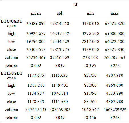
From the cryptocurrency data source Binance, we acquired a comprehensive dataset encompassing daily trading data on the price of Bitcoin and Ethereum. This dataset includes key variables such as opening prices, highest prices, lowest prices, closing prices, and trading volume. The temporal scope of this dataset spans from August 17, 2017, to October 31, 2023, providing a wide-reaching timeframe for analysis.
To evaluate an investor’s performance in Bitcoin and Ethereum trading, our analysis begins by calculating the daily gross return. This is done by purchasing one unit of cryptocurrency and holding it for one unit of time. The formula used for this calculation is 𝑟𝑡 = ln(𝑠𝑡/𝑠𝑡−1), where 𝑠𝑡 represents the price at time unit 𝑡.
Initially, we focus on examining the mean gains from cryptocurrency trading without considering transaction costs. In order to provide a comprehensive understanding of the returns, we present the summary statistics of returns for the BTC/USDT and ETH/USDT cryptocurrency pair in Table 1.
To ensure a rigorous evaluation, we proceed with an out-of-sample analysis. For this purpose, we divide the dataset into two distinct sections: the in-sample duration, which spans from Aug 17, 2017, to Dec 20, 2021, and the out-of-sample duration, which encompasses Dec 20, 2021, to Oct 31, 2023. This division allows us to assess the investment performance beyond the period used for model estimation, providing insights into the robustness of the findings.
Moving mean trading regulations are widely used in technical trading and can be constructed at various levels of complexity. The main objective of these regulations is to identify and capture patterns in the market, as well as to detect potential disruptions or the emergence of new patterns. One common and simple approach to moving mean trading is to use a single moving mean as an estimation of the local trend. When the value intersects with the moving mean, it serves as a trading signal to either initiate a new position or neutralize the current one. Traders often replace the value with a short-term moving mean in this type of regulation. For example, an upward disruption in the trend can be suggested when a short-moving mean intersects from below a long-moving mean. Conversely, a downward disruption in the trend can be indicated when the short-moving mean crosses the long-moving mean from above. Moving means can be classified into different categories based on their calculation periods. A moving mean with a calculation period of less than 20 days is considered a short-term moving mean, while one with a calculation period between 20 and 60 days is referred to as a medium-term moving mean. A moving mean with a calculation period longer than 60 days is recognized as a long-term moving mean. By utilizing moving means with different lengths, traders can assess the market trend over various time intervals. There are several methods available for calculating moving means, with the arithmetic moving mean being the most commonly used technique. This technique, also known as the simple moving mean, involves summing up a specific number of data points and dividing the sum by the number of points to calculate the average.
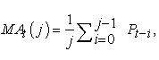 | (1) |
where j denotes the moving average period, MAt represents the moving average value on the t-th day, and Pt-i denotes the closing price on the (t-i)-th day.
A single moving average trading rule may be expressed as follows: If the asset’s daily closing value increases by at least x percent above MAt(q) and remains above it for a consecutive period of d days, it is seen as a signal to take a long position on the asset. The investor is advised to maintain this long position until the asset’s daily closing value decreases by at least x percent below MAt(q) and remains below it for d consecutive days. At this point, the investor should switch to a short position on the asset. Conversely, if the asset’s daily closing value decreases by at least x percent below MAt(q) and remains below it for d consecutive days, it serves as a signal to take a short position on the asset. The investor should maintain this short position until the asset’s daily closing value increases by at least x percent above MAt(q) and remains above it for d consecutive days. This is the point at which the investor should switch their position to a long one on the asset. The fundamental concept behind this trading rule is to capture price fluctuations that exceed a certain threshold in relation to the moving average, enabling investors to exploit potential trends and generate profits.
A modification that can be made to determine investment duration is to establish specific criteria based on the equity’s performance. If the daily closing value of the equity increases by at least x percent and exceeds the MAt(q) for a duration of d days, a long position in the equity should be taken for k days before selling. Conversely, if the daily closing value of the equity decreases by at least x percent below the MAt(q) and this decline persists for d days, a short position in the equity should be assumed for k days before being reversed. This modification does not consider any additional indications that may arise within the predetermined time frame. By implementing these criteria, investors can make informed decisions about the duration of their investments in the equity market. These criteria contribute to a systematic approach to investment management, facilitating a more structured and objective decision-making process.
A trading strategy known as the double moving average system can be defined as follows: When the moving average MAt(p) rises by a minimum of x percent above another moving average MAt(q) and maintains this upward trend for a period of d days, a long position on the asset is initiated. This long position is held until the MAt(p) drops by at least x percent below the MAt(q) and remains below it for d days. At this juncture, a short position is taken on the asset. Conversely, if the MAt(p) decreases by at least x percent below the MAt(q) and remains below it for d days, a short position is assumed on the asset. This short position is maintained until the MAt(p) increases by at least x percent above the MAt(q) and persists for d days. At this point, a long position is taken on the asset. It is important to note that the value of p is less than the value of q in this binary moving average trading approach. This strategy aims to exploit significant changes in the relative movements of two moving averages to determine entry and exit points for long and short positions in the financial market.
The prearranged adjustment of the double moving average trading concept for retaining intervals is as follows: If MAt(p) increases by at least x percent compared to MAt(q) and maintains this level for d days, then a bullish position on the underlying should be initiated for k days, followed by a return to equilibrium. Similarly, if MAt(p) decreases by at least x percent below MAt(q) and persists in this state for d days, then a bearish position on the underlying should be initiated for k days, followed by a return to neutrality.
After careful consideration of the preceding discussion, we have determined that the most suitable approach to implement is the EMAC (Exponential Moving Average Crossover) method. We will proceed with a retrospective analysis to evaluate its effectiveness. Consistent with the EMAC framework, we establish a set of parameter values for the fast span, ranging from 10 to 30 with increments of 4. Moreover, we conduct a systematic investigation across a range of values for the slow period, varying from 35 to 55 with increments of 4. This exhaustive exploration enables us to assess the performance of the EMAC approach across various scenarios and ascertain its efficacy in financial domains.
4.2. RSI StrategyOscillators play a crucial role in finance, serving as a widely employed technique referred to as the ”overbought/oversold” indicator. Despite its extensive usage, there is a lack of comprehensive academic investigation into this indicator. Oscillators function as measurement tools, specifically designed to identify situations when price movements have been excessively rapid in one direction, suggesting a potential correction in the opposite direction. Various types of oscillators exist, with the relative strength indicator (RSI) being a prominent example (Levy, 1967; Wilder, 1978). The RSI can be defined as
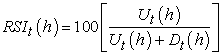 | (2) |
where Ut(h) denotes the cumulative ”rising action” over a specific time span h in the RSI computation. It reflects the price increase from one day’s closing price to the next day’s closing price, provided that the latter exceeds the former. Conversely, Dt(h) represents the cumulative absolute ”declining action” during the same timeframe. It quantifies the absolute price decrease from one day’s closing price to the next day’s closing price, when the latter is lower than the former.
It is noteworthy that certain RSI explanations define Ut(h) and Dt(h) in terms of the mean instead of accumulated up and down movements. Nevertheless, this approach is tantamount to the given definition as it involves division by the total number of days, and this factor cancels out when computing the RSI.
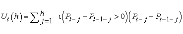 | (3) |
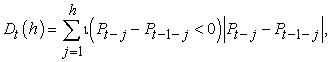 | (4) |
where the signal variable 𝜄(·) takes the value one when the assertion in parentheses is true and zero otherwise.
The RSI serves the purpose of evaluating the strength of ascending and descending movements in the market, thereby assessing the equilibrium between buyers and sellers. If the upward momentum dominates, the calculated RSI indicator will increase, indicating a stronger bullish market trend. Conversely, if the downward momentum prevails, the RSI indicator will decrease, signaling a stronger bearish market trend. Consequently, the RSI can be utilized as a tool to assess the strength of market trends.
The RSI is a numerical indicator ranging from 0 to 100, with 50 serving as the equilibrium point. Typically, a value between 30 and 70 is considered normal and implies a balanced trading state. However, readings above 80 or below 20 indicate a reduced likelihood of profitable trading opportunities. To enhance its predictive power, analysts frequently utilize different time frames for the RSI. For example, the 6-day, 12-day, and 24-day lines are commonly employed to analyze short, medium, and long-term market trends, respectively. By evaluating the RSI value within these time frames, one can gather insights into the strength of both long and short positions, as well as the direction of the prevailing trend.
Specifically, the RSI value of 50 serves as a significant demarcation point between long and short positions. If the RSI consistently remains above 50, experts interpret this as indicative of a strong long position. Conversely, a sustained RSI value below 50 points to a strong short position. Additionally, monitoring the upward or downward trend of the RSI line further reveals changes in the strength of both long and short positions.
This principle is typically implemented by identifying specific conditions that signal a potential opportunity to initiate or terminate a transaction. To be more precise, if the RSI value at time period RSIt(h) exceeds 50 + v for a minimum of d consecutive days and subsequently falls below 50 + v, it suggests a favorable scenario for engaging in short-selling the asset. On the other hand, if RSIt(h) drops below 50 - v for at least d days and then rises above 50 - v, it indicates a suitable situation for assuming a long position in the asset.
By adhering to this wave-like strategy, market participants can attempt to exploit potential changes in price dynamics or shifts in market momentum.
A modification to the traditional RSI trading rule introduces a predefined time period during which a position must be held. In this revised rule, if RSIt(h) exceeds 50 + v for at least d consecutive days and then falls below 50 + v, it is recommended to assume a short position on the asset for a duration of k days, followed by neutralizing the position. Conversely, if RSIt(h) falls below 50 - v for at least d consecutive days and then rises above 50 - v, it is advised to assume a long position on the asset for a duration of k days, followed by neutralizing the position. This modification aims to incorporate specific criteria for entry and exit points based on RSI movements to enhance trading strategies. The use of a specified holding period helps determine the optimal timing for assuming positions, potentially leading to more successful outcomes.
When the RSI exceeds 50 + v or falls below 50 - v, it signifies overbought or oversold conditions in the market. However, the generation of a trading indicator based on the RSI does not transpire at this stage. Instead, the trading indicator materializes when the RSI exits the excessively bought or sold area. This implies that when the RSI traverses 50 + v from above or crosses 50 - v from below, it signals the creation of a trading indicator. The rationale behind this approach is that the asset may sustain these extreme conditions for an extended duration. In fact, there is even a possibility for these conditions to be momentarily intensified.
In view of the previously mentioned preamble, our subsequent action entails choosing the RSI approach and assessing its effectiveness through the implementation of a historical backtesting procedure. To evaluate the RSI approach, we designate the RSI duration as 14.
Subsequently, we proceed to examine a range of values for the upper RSI limit, ranging from 70 to 90, with an increment of 4. Similarly, we establish a range for the lower RSI limit, varying from 20 to 40, with an increment of 4. Through this comprehensive exploration of different RSI values, our aim is to assess the performance of the approach.
4.3. Bollinger Bands StrategyEfforts aimed at establishing benchmarks for trading, specifically those based on support and resistance levels, seek to identify key thresholds at which the value of a financial instrument encounters obstacles in increasing (referred to as a resistance threshold) or decreasing (known as a support threshold). These benchmarks operate under the assumption that when a support or resistance threshold is surpassed, there will be significant movement in the corresponding direction. Support-resistance trading benchmarks share similarities with filter benchmarks, with the only distinction being that a trading signal is generated when the value surpasses a support or resistance threshold by a specific percentage, as opposed to surpassing a recent high or low point.
In order to effectively determine support and opposition levels, it is crucial to establish them beforehand. One commonly used methodology involves defining an opposition level as the highest closing price among the previous j cessation prices, while a support level is defined as the lowest closing price among the same set of j prior cessation prices. Once these levels have been identified, a trading strategy can be implemented. If the daily closing price of the asset increases by at least x percent beyond the highest prior closing price within the j previous cessation prices and maintains this upward trend for a duration of d days, it is advisable to take a long position in the asset. Conversely, if the daily closing price of the asset decreases by at least x percent below the lowest prior closing price within the j previous cessation prices and sustains this level for d days, it is recommended to take a short position in the asset. By following these guidelines, investors can make informed decisions about the appropriate times to go long or short on an asset.
The prearranged retention period version of the support-resistance principle is analogous to the corresponding filtration principle. Under this version, if the daily closing amount of the investment increases by at least x times over the maximum of the previous j closing amounts and remains for d consecutive days, a long position in the investment is assumed for k days, followed by closing the position. Conversely, if the daily closing amount of the investment decreases by at least x times below the minimum of the previous j closing amounts and remains for d consecutive days, a short position in the investment is assumed for k days, followed by closing the position.
An alternative method for determining the levels of hindrance and support is the Bollinger Band, developed by technical trader John Bollinger and commonly utilized in technical analysis. The hindrance and support levels are represented as n deviations, either positive or negative, from a simple moving average (SMA) of a security’s price. The trading guidelines associated with Bollinger Bands are similar to those mentioned earlier.
Given the discourse mentioned above, we opt for the specific Bollinger Bands strategy and carry out a retrospective analysis to assess its effectiveness. To incorporate the Bollinger Bands approach, we consider a range of durations from 15 to 30, increasing by intervals of 3. Additionally, we investigate the devfactor across three different magnitudes: 1.0, 2.0, and 3.0. This comprehensive examination enables us to comprehensively evaluate the efficiency of the Bollinger Bands strategy.
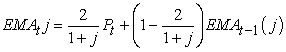
4.4. MACD StrategyThe moving average trading strategy is a frequently utilized technique in finance. It involves calculating the arithmetic average of prices over a specific period. However, this strategy has certain limitations. Firstly, it suffers from lag, meaning that it may not accurately reflect the current market conditions. Additionally, it assigns equal weight to all values, regardless of their proximity to the current moment. To overcome these drawbacks, finance professionals introduced a more sophisticated indicator known as the Moving Average Convergence Divergence (MACD). The MACD utilizes exponential moving averages (EMA) instead of simple moving averages. This helps address the lag problem associated with the traditional approach. Furthermore, the use of EMA allows the MACD to reduce the generation of frequent trading signals from short backtesting periods.
The calculation of the MACD involves subtracting a long-term EMA, typically measured over 26 days, from a short-term EMA, typically measured over 12 days. This difference is referred to as DIF. Additionally, the MACD Signal Line, known as DEA, is derived using the MACD’s EMA. By incorporating EMA and considering different time periods, the MACD provides a more refined and accurate approach to analyzing trading strategies.
 | (5) |
 | (6) |
 | (7) |
where n denotes the EMA period, which is a key parameter that determines the weightage of recent prices in the calculation.
The bar of MACD serves as a measure of the distance between the MACD and its signal line. An optimistic disparity between the DIF and DEA indicators leads to a favorable value for the MACD bar, suggesting a bullish market. Conversely, an unfavorable difference between the DIF and DEA indicators causes the MACD bar to adopt an adverse value, indicating a bearish market. Additionally, the contraction and inversion of the MACD bar can be used as a technique to identify potential trading opportunities. This technique involves closely monitoring the changes in the MACD bar as it can provide valuable insights for traders. By observing the variations in the MACD bar, traders can potentially determine the optimal time to enter or exit a specific market position. Consequently, comprehending and analyzing the behavior of the MACD bar can contribute to more informed and strategic investment decisions.
Furthermore, in situations where the DEA trendline deviates from the candlestick chart, with the DEA line reaching a new high while prices do not, or vice versa, this suggests a potential market reversal. It is important to note that the reversal does not necessarily entail a V-shaped or inverted V-shaped pattern, but may instead involve a more extensive shift in the overall trend.
A standard MACD trading rule can be defined as follows: if DIF increases by at least x percent above the DEA and persists above this level for d days, take a long position in the asset, and the long position should be maintained until DIF decreases by at least x percent below the DEA and remains below this threshold for d days, indicating a reversal in market momentum. At this point, it is recommended to switch to a short position in the asset. On the contrary, if DIF declines by at least x percent below the DEA and persists below this level for d days, it is advisable to initiate a short position in the asset. This short position should be held until DIF increases by at least x percent above the DEA and remains above this threshold for d days, indicating a potential market upturn. This trading strategy allows investors to take advantage of changes in market momentum and adjust their positions accordingly, potentially benefiting from favorable market conditions.
Based on the aforementioned introduction, we have chosen to use the MACD methodology and evaluate its effectiveness through a retrospective analysis. In relation to the MACD strategy, we investigate different options for the fast period, ranging from 10 to 25 with a step size of 5. The slow period is defined within a range of values from 25 to 40, also with a step size of 5. The signal period is specified over a range of values from 6 to 12, with a step size of 3. We determine the simple moving average duration to be 30. The direction period is chosen as 10.
Logarithmic returns play a crucial role in capturing the rapid pace at which the price is rising. Unlike other metrics that focus on the percent of price change for each sub-period, logarithmic profits provide insights into the exponent of its natural growth during that time.
The equation to calculate the cumulative composite yield is provided as follows:
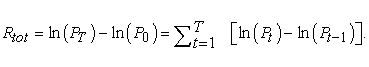 | (8) |
The arithmetic mean represents the average of logarithmic returns, which is measured by:
 | (9) |
In practical scenarios, it would be advantageous for this indicator to serve as a universally comparable annual return percentage. To achieve this objective, we employ a standardization approach for our return metric by converting it into an average annualized return. This conversion is carried out as follows:
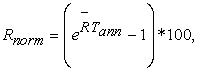 | (10) |
where 𝑇𝑎𝑛𝑛 denotes the number of sub-periods in one year: 12 for monthly, 52 for weekly, and 252 for daily configurations.
5.2. Sharpe RatioThe Sharpe Ratio is widely used and firmly established as a performance gauge in the finance industry. It provides an evaluation of the average excess income obtained for each unit of uncertainty, where uncertainty is measured by the standard deviation of excess incomes. By examining the relationship between returns and volatility, the Sharpe Ratio offers valuable insights into the performance of investments when adjusting for uncertainty. A higher ratio indicates better performance adjusted for volatility, suggesting that the investment has generated higher incomes compared to the level of risk taken. In this study, we focus on the ex-post Sharpe ratio (SR) as our chosen measure.
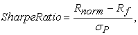 | (11) |
where 𝑅𝑛𝑜𝑟𝑚 refers to the total annualized returns of the strategy, 𝑅𝑓 denotes the risk-free rate, and 𝜎𝑃 denotes the algorithm volatility of the strategy.
5.3. Max DrawdownMax drawdown is defined as the largest percentage decline from a previous peak to a subsequent low, making it a key indicator for assessing the downside risk involved in an investment strategy. By understanding max drawdown, investors gain insights into potential losses that they may encounter during turbulent market conditions. Managing max drawdown is essential for investors seeking to protect their capital, minimize losses, and make well-informed investment decisions.
 | (12) |
where 𝑃𝑖, 𝑃𝑗 are the total value of the portfolio on day i and day j, respectively, and 𝑗 > 𝑖. Here we use the length of the period and value in percentage of max drawdown as metrics.
One crucial aspect of this research is examining potential data-snooping bias. The significance of this lies in the absence of strict theoretical restrictions when constructing technical trading strategies. Consequently, researchers have the flexibility to choose various parameters, resulting in multiple alternative hypotheses for the statistical inferences under consideration. To ensure the reliability and validity of our findings, it is essential to determine whether the profitable trading strategies identified through specification search genuinely exhibit predictive superiority compared to a given benchmark model. However, achieving this task within the framework of classical statistical inference presents significant challenges.
Classical statistical inference relies on rejecting the null hypothesis when the likelihood of the observed data under the null hypothesis is low. However, when exploring different trading strategies, the number of hypotheses being implicitly tested increases as underperforming models or rules are discarded. This leads to the problem of multiplicity, where the higher the number of hypotheses being tested, the greater the likelihood of encountering rare events and erroneously rejecting the null hypothesis of interest in each competing model or trading rule (referred to as Type I error). The robust performance of models identified through specific searches and subsequent rejection of individual null hypotheses do not guarantee predictive superiority over a given benchmark model. Instead, their apparent success may be attributed to the extensive specification search conducted. In our specific analysis, where we evaluate up to 83 different variants of technical trading strategies, skeptics might argue that it would be surprising if we did not find any strategies that performed well.
Applied scholars are well acquainted with the challenge of information excavation or the overfitting of data. This issue, which is also known as information exploring, has a longstanding presence in applied finance, with notable advancements made in recent times (Leamer 9 and references therein).
In this study, we examine a collection of 𝐾 performance measurement vectors denoted by  . Each component 𝐷𝑘 represents a specific performance measurement, such as average return or Sharpe ratio, for the 𝑘𝑡ℎ strategy where 𝑘 = 1, 𝐾. Traditionally, researchers have often opted for selecting the maximum component of the performance vector, denoted as
 , and testing the null hypothesis that this component is equal to zero. This approach allows researchers to investigate the potential significance of the highest-performing strategy within the set of strategies being considered.
 | (13) |
A trial of the null hypothesis using Equation (13) is referred to as an ”individual test.” The nominal t-statistic for this individual test is calculated as follows:
 | (14) |
where  denotes the standard deviation of the variable
  . Once these values are obtained, the computation of the nominal p-value relies on the cumulative distribution function.
White 10 posits that conventional statistical inference methods fail to account for the fact that  represents the highest element in D, resulting in an asymmetrical statistical distribution. The selection of
  depends on its maximum value following a comprehensive investigation among a potentially extensive set of 𝐾 alternatives. Consequently, the specified significance level assigned to the test will underestimate the actual probability of committing a Type I error. In other words, the test is biased toward rejecting the null hypothesis due to data-snooping. This limitation highlights the need for alternative methodologies that address the bias caused by data-snooping during hypothesis assessments.
The “reality check” test introduced by White 10 is a valuable tool for researchers in the finance field to address potential data snooping concerns and validate their findings. This test utilizes bootstrapping, a resampling technique that creates multiple samples emulating the original dataset, to evaluate a composite null hypothesis formed on the basis of the joint distribution of all elements of the vector D. By generating an empirical distribution through bootstrapping, the test allows for a comprehensive analysis of the interdependencies between variables and provides a more robust assessment of hypotheses. The utilization of this test contributes to the advancement of rigorous and reliable research in finance, providing researchers with a means to address data snooping concerns and enhance the validity of their findings.
 | (15) |
where 𝐷𝑘 denotes the mean return or Sharpe ratio of the 𝑘𝑡ℎ strategy. To ensure an accurate assessment of the significance levels of gains obtained from these strategies, we adopt a multiple-testing technique. We utilize the bootstrap reality check methodology as suggested by White 10 to facilitate this evaluation. In this methodology, we demonstrate the determination of p-values for the reality check using daily data as an illustrative example.
1. We compute the daily return matrix A, in which each element 𝐴𝑘𝑡 denotes the daily return of the 𝑘𝑡ℎ strategy in each day 
2. We resample A using the stationary bootstrap method of Politis and Romano 11, with pre-specified parameter set Y, for 𝐵 times, and label each resample as  .
.
3. For each strategy 𝑘, we compute its performance metric (mean return or Sharpe ratio), 𝐷𝑘, based on A and 𝐷𝑘𝑏 based on A𝑏.
4. Now set  and
and  and set
  and
and  for
for 
5. Denote the sorted values of  as
as  Find 𝑋 such that
  . The bootstrap reality check p-value can be calculated as
The effectiveness of the reality verification examination can be compromised when irrelevant options are included, as stated by Hansen 12. The presence of these inconsequential alternatives weakens the ability of the examination to refute the incorrect null hypothesis. To address this issue, it is suggested to studentize the examination statistic and incorporate a sample-specific null distribution to identify the relevant alternatives. This approach involves a sequential examination, which expands upon White’s reality verification examination. The sequential methodology incorporates the contributions of Hansen 12, Romano and Wolf 13, and Hsu, Hsu, and Kuan 14. To begin, the alternative propositions for the null hypothesis in Equation (15) are specified as:
 | (16) |
The rejection of the 𝑘𝑡ℎ singular void notion indicates that the 𝑘𝑡ℎ technological methodology is highly profitable when all other notions are taken into account, thereby avoiding data snooping bias. We define the sequential analysis with a specified Type I error level 𝛼0 over a given time period  as elaborated below{2}:
1-3. The first three steps are the same as that of calculating reality check p-values.
4. We construct an empirical null distribution for the test statistics as follows:
(a). For each 𝑏, compute
 | (17) |
where  represents the indicator function of event 𝑃 and 𝜎𝑘 denotes the standard deviation of the original daily return series of the 𝑘𝑡ℎ strategy. The bound
  is proposed by Hansen 12 to re-center the distribution for D to avoid the bias driven by too many “bad” strategies.
(b). Collect and rank all  in descending order and then collect its
  quantile as
  .
.
5. We compare each strategy’s  to
to  and treat the 𝑘𝑡ℎ null hypothesis as rejected at the
  step if
  , following Romano and Wolf 13. We record all information of these rejected strategies and label then rejected at the 𝑖𝑡ℎ step. Then, restart from Step 5, let 𝐷𝑘 = 0 and 𝐷𝑘𝑏 = 0 for all rejected hypotheses 𝑘, and change the loop indicator from 𝑖 to 𝑖 + 1. However, if no strategy is rejected given
  , i.e.
  for the remaining 𝑗, then stop and go to Step 7.
6. Finally, restore the original 𝐷𝑘 from A and estimate each technical rule’s marginal p-value, 𝑝𝑘, as the percentile of  in the last
  as an empirical null distribution.
7. Compare each technical rule’s  to
to  . If
. If  , we claim that 𝑘𝑡ℎ strategy is profitable in the sample period at the significance level of 𝛼0. When there exists at least one profitable strategy in the sample period, we claim that technical trading is profitable at the significance level of
  and the stepwise test p-value is 1 −
  .
.
It is imperative to adopt precise parameter values in our empirical analysis in order to ensure rigor and comparability with the existing literature. We set the significance level, 𝛼0, at 0.05, which implies that we only consider results with a confidence level of 95% or higher. Following the literature, we set 𝑄 = 0.9 and 𝐵 = 1000.
It is important to highlight the significance of data-snooping tests in evaluating the credibility of a strategy’s profitability. Although a strategy may demonstrate positive profit in our analysis, there is a possibility that its success is merely due to chance rather than its true effectiveness. To mitigate the risk of false discoveries, we subject all strategies to rigorous data-snooping tests.
In this section, We investigate the profitability of technical trading strategies during both the in-sample and out-of-sample periods. The analysis is conducted with a starting cash amount of 100,000, and the maximum buying capacity and the maximum selling capacity are set to 1. To incorporate transaction costs, we designate a slippage value of 0.001 and a commission rate of 0.0003. Our trading choices rely exclusively on the closing prices from the preceding trading day. Notably, Fractional trading and short selling are not permitted.
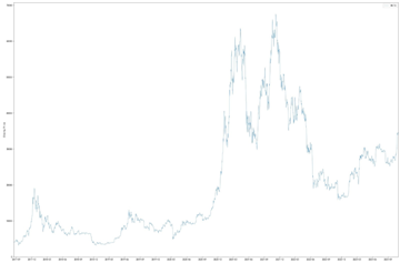
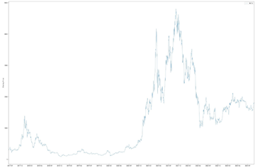
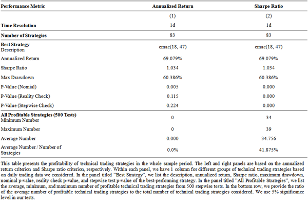
Table 2 presents the test results for the entire sample period, evaluating different groups of technical trading strategies based on two performance criteria: annualized return and Sharpe ratio. The analysis focuses on two sets of indicators derived from the data snooping test. Firstly, we examine the performance metrics and associated p-values of the best strategy. Secondly, we assess the number of profitable strategies that produce significantly positive performance metrics. The tests are conducted with a nominal significance level of 5%. The “Description” row displays the best strategy based on daily trading data, while the subsequent rows provide the corresponding nominal p-value, reality check test p-value, and stepwise test p-value.
An example presented in column (1) reveals that the best strategy is emac(18, 47), representing the EMAC strategy with a fast period of 18 and a slow period of 47. This optimal strategy shows an annualized return of 69.079%, a Sharpe ratio of 1.034, and a maximum drawdown of 60.386%. However, the nominal p-value of 0.005, the reality check test p-value of 0.115, and the stepwise test p-value of 0.224 indicate that the annualized return of the strategy is not statistically significant at a 5% level.
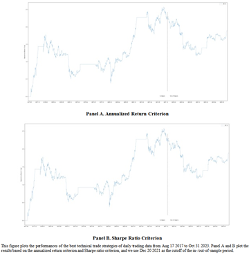
To gain further insights into the performance, Figure 3 illustrates the cumulative log returns of the best-performing technical trading strategies based on daily trading data.
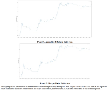
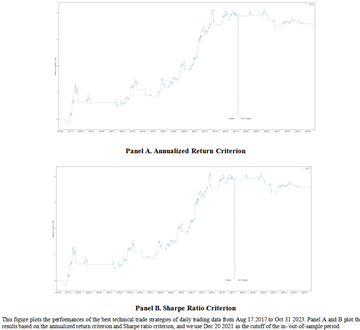
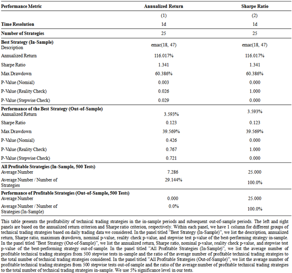
The analysis in Table 3 unveils the findings of the Exponential Moving Average Crossover (EMAC) approach in both the in-sample and out-of-sample examinations. The left and right sections of the table are based on the evaluation of annualized returns and Sharpe ratio as measures of performance, respectively. In the section referred to as ”Best Strategy (In-Sa”, we present a comprehensive account of the explanation, annualized return, Sharpe ratio, maximum drawdown, and the nominal, reality check test and stepwise test p-values of the most successful technique in the in-sample analysis. In the section denoted as ”Best Strategy (Out-of-Sa”, we provide details regarding the annualized return, Sharpe ratio, and the nominal, reality check test and stepwise test p-values of the top-performing technique in the out-of-sample analysis. In the subsequent section referred to as ”All Profitable Strategies (In-Sample, 500 Tests)”, we perform the data snooping tests 500 times to mitigate the bias in bootstrapping due to sampling. In the final section titled ”Performance of Profitable Strategies (Out-of-Sample, 500 Tests)”, we enumerate the average quantity and proportion of approaches that consistently yield profits during the out-of-sample period. As illustrated in column (1), for instance, the most effective EMAC technique exhibits a fast period of 18 and a slow period of 47 as its parameters. This optimal methodology yields an annualized return of 116.017%, a Sharpe ratio of 1.341, and a maximum drawdown of 60.386%. Although the return on investment of the technique is statistically significant at a 5% significance level, as indicated by the p-values below the threshold of 5%, its outstanding performance in the in-sample analysis does not persist in the subsequent out-of-sample period, with an insignificant annualized return of 3.593% that fails to reject the null hypothesis. If financiers adopt the optimal technique based on the in-sample period, they may generate profits in the out-of-sample period, but these profits are likely attributable to chance rather than any inherent merit in the methodology leading to the results. The cumulative log returns of the top-performing technical trading methodologies based on daily trading data are depicted in Figure 4.
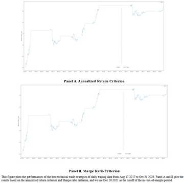
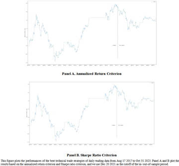
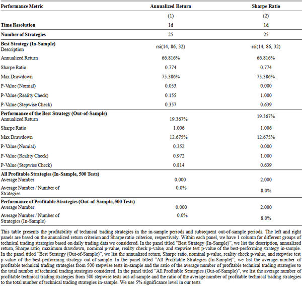
In Table 4, we present the examination outcomes for the RSI strategy in both the training and testing samples. The performance conditions used for evaluation are the annualized benefit and the Sharpe ratio, which are analyzed in the left and right sections, respectively. For example, column (1) demonstrates the performance of the most successful RSI approach with specific parameters, such as an RSI period of 14, an RSI upper of 86, and an RSI lower of 32. This optimal approach yields an annualized benefit of 66.816%, a Sharpe ratio of 0.774, and a maximum drawdown of 75.386%. However, despite these impressive results, the approach does not exhibit exceptional performance in the sample period, as its average annualized benefit is statistically insignificant and cannot reject the null hypothesis. Moreover, it fails to generate significant profits during the subsequent testing period, with an annualized benefit of 19.367% that fails to reject the null hypothesis. These findings highlight the need for a more dependable and sustainable approach to consistently generate returns. To provide a further visual representation of our findings, we plot the cumulative log returns of the most successful technical trading approaches based on daily trading data in Figure 5. This graphical illustration enhances our understanding of the performance of the RSI approach and its comparison to other approaches.
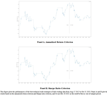
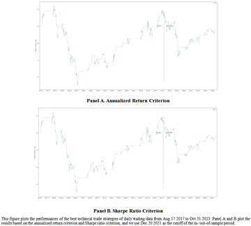
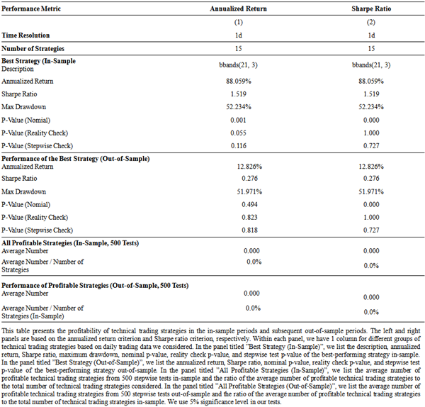
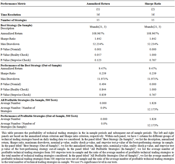
The results of the examination for the Bollinger Bands tactics, both in the sample and out of the sample, are displayed in Table 5. The first part of the table focuses on the compounded yearly yield as a performance measure, while the second part examines the Sharpe ratio. Column (1) highlights the most effective Bollinger Bands tactic, which has a term of 21 and a devfactor of 3. This tactic achieves a compounded yearly yield of 88.059%, a Sharpe ratio of 1.519, and a maximum loss of 52.234%. However, when evaluating its effectiveness in the out-of-sample period, it fails to generate significant gains, with a compounded yearly yield of only 12.826%. Additionally, the p-values associated with the tactic’s performance do not reject the null hypothesis. Therefore, it can be concluded that the Bollinger Bands tactic proves to be ineffective in both the in-sample and out-of-sample periods. Figure 6 provides a visual representation of the cumulative logarithmic yields of the top-performing technical trading tactics based on daily trading data.
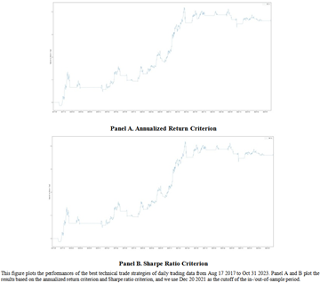
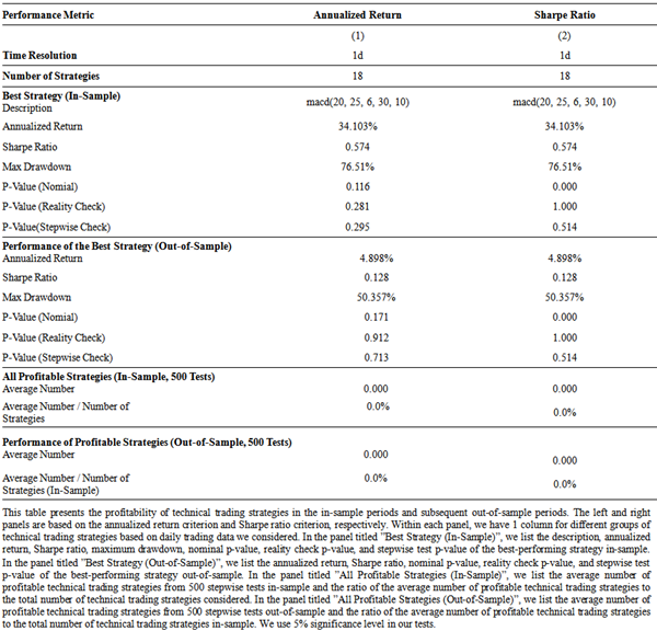
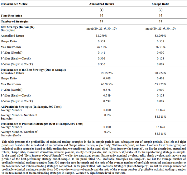
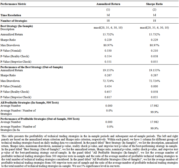
Table 6 presents the examination findings for the MACD approach, both within and beyond the sample set. The benchmarks of achievement that have been assessed include the standardized yearly profit and the Sharpe measure. In regards to the specific attributes of the most successful MACD approach highlighted in the example, it produces an average standardized yearly profit of 34.103%, a Sharpe measure of 0.574, and a maximum drawdown of 76.51%. However, this approach does not demonstrate notable performance within the in-sample timeframe and fails to generate gains in the subsequent out-of-sample timeframe. This lack of efficacy suggests limitations in the methodology. Additionally, Figure 7 illustrates the cumulative logarithmic returns of the most successful technical trading approaches utilizing daily trading data.
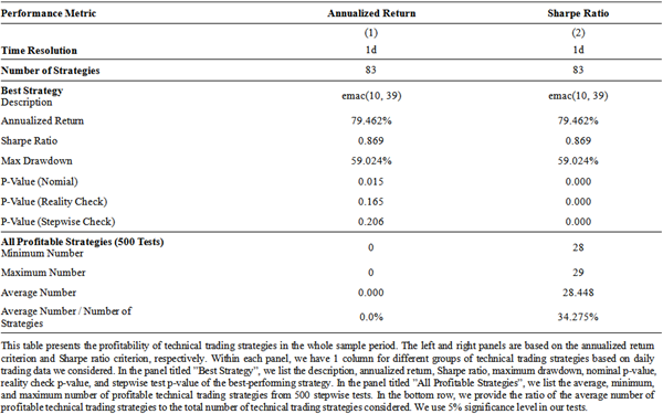
The results of the examination considering the whole sample period are presented in Table 7, which displays the performance criteria of annualized gain and Sharpe ratio. The table is divided into two sections, with one section representing different sets of methodologies based on the examined data. The study primarily focuses on two categories of indicators generated from a data snooping examination. The first category includes performance metrics and associated p-values of the most superior methodology, while the second category examines the number of advantageous methodologies that generate significantly positive performance metrics. A customary significance level of 5% is utilized in the analyses.
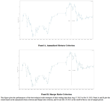
To illustrate, in column (1), the EMAC methodology with a swift period of 10 and a tardy period of 39 is identified as the most outstanding methodology. This methodology demonstrates an average annualized gain of 79.462%, a Sharpe ratio of 0.869, and a maximum drawdown of 59.024%. However, it does not exhibit exceptional performance throughout the entire sample duration, as its average annualized gain is considered insignificant and unable to reject the null hypothesis. The corresponding p-values are as follows: customary p-value = 0.015, reality check examination p-value = 0.165, and stepwise examination p-value = 0.206.
In order to visualize the outcomes of the most superior technical trading methodologies based on everyday trading data, Figure 8 presents the cumulative log returns.
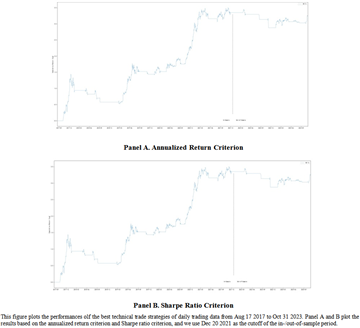
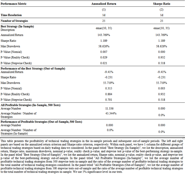
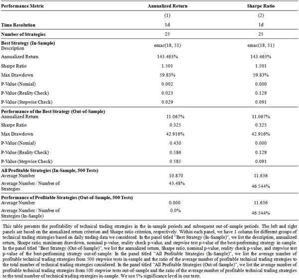
Test results for the EMAC approach are presented in Table 8, providing a detailed analysis of performance in both the in-sample and out-of-sample periods. The performance metrics used for evaluation are the annualized gain and Sharpe ratio for the left and right segments, respectively. For instance, results in column (1) demonstrate that the EMAC approach, with a prompt phase of 10 and a sluggish phase of 35, outperforms all other strategies. It achieves an annualized gain of 143.769%, a Sharpe ratio of 1.189, and a maximum drawdown of 58.626%. The approach exhibits exceptional performance in the in-sample interval, with the mean annualized gain being statistically significant and rejecting the null hypothesis at a 5% significance level. However, the annualized gain of -9.41% in the subsequent out-of-sample interval is no longer statistically significant, suggesting that the exceptional performance of the optimal approach does not persist. If investors were to follow the superior-performing approach from the in-sample interval, they may generate profits in the out-of-sample interval, but these profits are likely due to chance rather than any inherent merit in the technique employed, as demonstrated by the lack of statistical significance. To provide a further visual representation, we plot the cumulative log gains of the superior-performing technical trading approaches based on daily trading data in Figure 9.
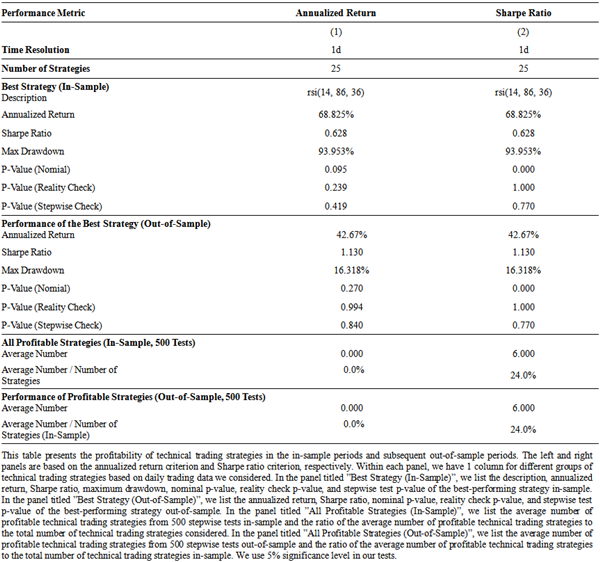
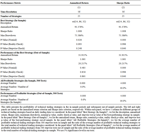
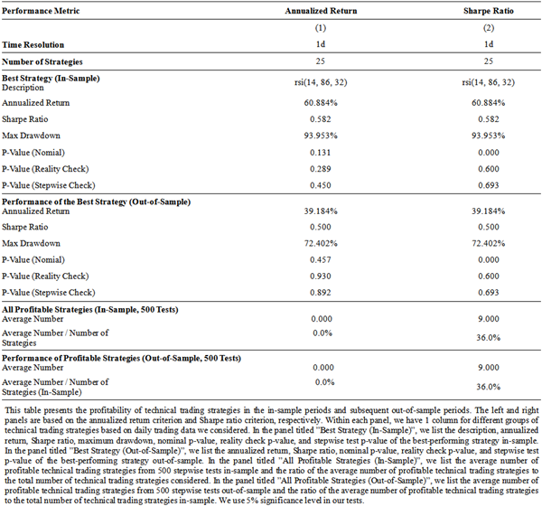
Table 9 showcase results of the RSI strategy for both the in-sample and out-of-sample periods. The left and right sections are based on annual profit and the Sharpe ratio, respectively, as benchmarks for performance. For example, column (1) shows that the RSI strategy with parameters of an RSI period of 14, RSI upper of 86, and RSI lower of 36 outperforms all other techniques, resulting in an annual profit of 68.825%, a Sharpe ratio of 0.628, and a maximum decline of 93.953%. However, this technique does not demonstrate exceptional performance in the in-sample period as its mean annual profit is negligible and cannot reject the null hypothesis. Furthermore, it also fails to generate profits in the subsequent out-of-sample period, with a negligible annual profit of 42.67% that fails to reject the null hypothesis. Overall, the technique fails to generate profits in both the in-sample and out-of-sample periods, indicating a lack of efficacy in the approach. We present the cumulative logarithmic returns of the most advantageous technical trading techniques based on daily trading data in Figure 10.
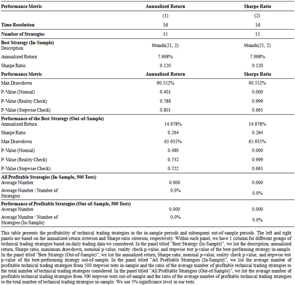
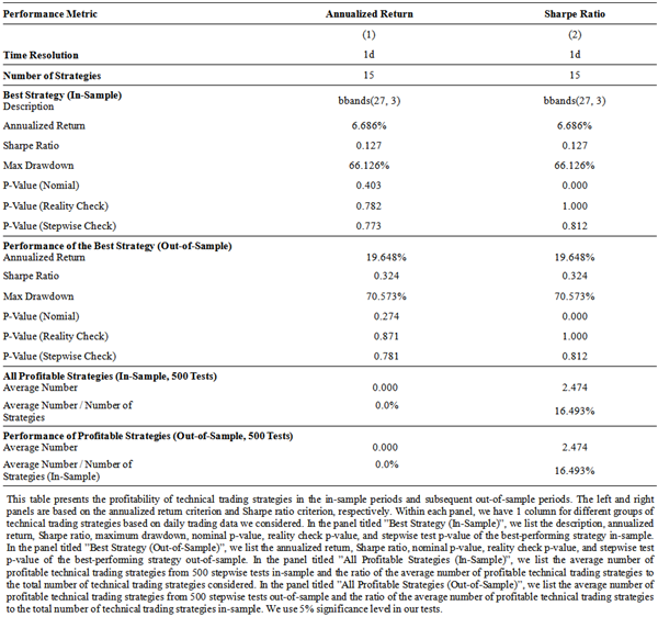
Table 10 presents the in-sample and out-of-sample assessment outcomes for the Bollinger Bands technique. The previous section focuses on the annual return, while the following section evaluates the Sharpe ratio as a performance measure. More specifically, column (1) showcases the most favorable Bollinger Bands approach with a duration of 21 and a devfactor of 2 as its parameters. This ideal approach yields an annualized return of 7.998% and a Sharpe ratio of 0.12, accompanied by a maximum drawdown of 90.552%. However, the approach’s unsatisfactory performance in the in-sample period, as indicated by the p-values, is echoed in the out-of-sample period, with an insignificant annualized return of 14.978% and p-values that fail to reject the null hypothesis. Therefore, the lack of profitability of the approach in both the in-sample and out-of-sample periods highlights the need for a more reliable and sustainable approach to generate consistent returns. To better illustrate the performance of the most effective technical trading approaches based on daily trading data, the cumulative log returns are plotted in Figure 11.
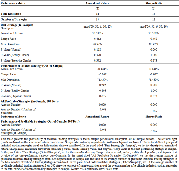
By examining the in-sample and out-of-sample test results, Table 11 provides a comprehensive evaluation of the MACD strategy’s performance. Upon examination of the specific details of the best-performing MACD strategy, it becomes evident that its parameters play a crucial role in determining its performance. The strategy has a fast period of 20, a slow period of 35, a signal period of 6, an SMA period of 30, and a direction period of 10. It generates an average annualized return of 33.508% and a Sharpe ratio of 0.462. However, despite these seemingly impressive figures, the strategy fails to achieve significant performance in both the in-sample and out-of-sample periods. In fact, it fails to reject the null hypothesis, indicating a lack of statistical significance and profitability. These findings suggest caution should be exercised when considering the MACD strategy, as it may not be effective in generating profits. In Figure 12, the cumulative log returns of the best-performing technical trading strategies are displayed, providing a visual representation of the results.
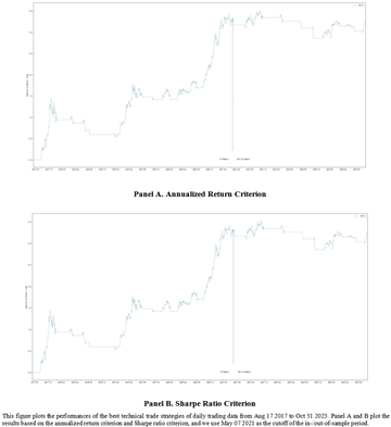
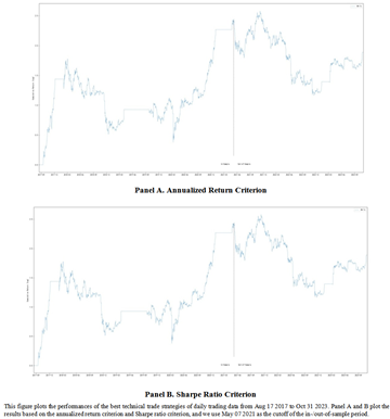
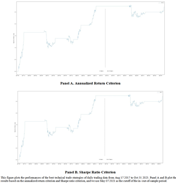
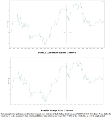
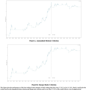
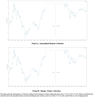
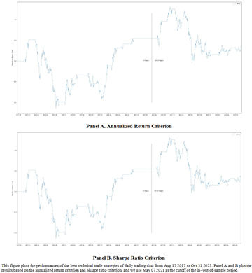
This section presents the outcomes of a number of robustness checks conducted to validate the accuracy and consistency of our analysis. One criticism raised against our utilization of December 20, 2021, as the cutoff date in our analysis, is that our findings could be attributed to mere chance. In order to address this concern and provide a more comprehensive assessment, we perform a robustness check by employing May 07, 2021, as the cutoff date for both the in-sample and out-of-sample periods. The results of this robustness check can be found in the Appendix. Importantly, these results align with our previous findings based on December 20, 2021, thus further affirming our conclusion regarding the efficiency of the cryptocurrency market.
This additional analysis serves to reinforce the validity of our conclusion and offers further substantiation of the robustness of our findings. By incorporating the alternative cutoff date, we ensure a comprehensive assessment of our analysis. The results obtained from this robustness check provide additional support for our initial findings, consolidating the reliability and credibility of our research results. Therefore, the inclusion of this supplementary analysis enhances the overall value of our study, contributing to the advancement of knowledge in the field of cryptocurrency market efficiency.
In this paper, our objective is to examine the out-of-sample profitability of in-sample lucrative specialized trading strategies using extensive amounts of data from the BTC/USDT and ETH/USDT cryptocurrency pairs. We utilize a timeframe ranging from August 2017 to October 2023 to conduct our analysis. By formulating various technical trading strategies based on indicator selection and time resolution, we are able to draw significant conclusions regarding the effectiveness of these strategies in an out-of-sample scenario.
After carefully considering the issue of data-snooping bias and taking steps to correct it, we find that specialized trading strategies that were identified as profitable prior to December 2021 generally exhibit a lack of profitability in the subsequent out-of-sample period. This suggests that these strategies may not be as reliable or effective when applied to new data. To ensure the robustness of our findings, we evaluate the performance of the best-performing specialized trading strategy using different performance metrics. Even when considering the alternate date of May 07, 2021, as the dividing point between the in-sample and out-of-sample periods, our conclusions remain consistent. This reinforces the notion that these in-sample profitable strategies may not yield consistent profits when applied to new or unseen data.
The main contribution of this paper is to point out that it is difficult to choose specialized trading strategies with out-of-sample profitability. While certain strategies may appear lucrative based on historical data, it is crucial to validate their performance in real-time market conditions to avoid potential pitfalls and make more accurate investment decisions. Consequently, our research lends support to the efficient market hypothesis within the cryptocurrency market, suggesting that the discovery of profitable strategies through backtesting does not guarantee their future effectiveness. In other words, the ability to generate profits from technical trading strategies in hindsight does not necessarily imply their potential for learning and replication in a forward-looking manner.
{1}. Data-snooping bias occurs when researchers only conduct individual examinations without considering the need to test all models or rules collectively for their significance.
{2}. In technical terms, the error we aim to control for in this multiple testing framework is the family-wise error, which is the probability of rejecting at least one valid null hypothesis. For instance, if we set a 5% significance level in the analysis, we expect a 5% chance of erroneously rejecting any alternative hypothesis (i.e., identifying any inefficient approach as profitable).

| [1] | Tam, Phan Huy, and Nguyen Thanh Cuong, 2018, Effectiveness of investment strategies based on technical indicators: Evidence from vietnamese stock markets, Journal of Insurance and Financial Management 3, 55–68. | ||
| In article | |||
| [2] | Kwon, Ki-Yeol, and Richard J Kish, 2002, Technical trading strategies and return predictability: Nyse, Applied Financial Economics 12, 639–653. | ||
| In article | View Article | ||
| [3] | Ratner, Mitchell, and Ricardo PC Leal, 1999, Tests of technical trading strategies in the emerging equity markets of latin america and asia, Journal of Banking Finance 23, 1887–1905. | ||
| In article | View Article | ||
| [4] | Resta, Marina, Paolo Pagnottoni, and Maria Elena De Giuli, 2020, Technical analysis on the bitcoin market: trading opportunities or investors¡¯ pitfall? Risks 8, 44. | ||
| In article | View Article | ||
| [5] | Fousekis, Panos, and Dimitra Tzaferi, 2021, Returns and volume: Frequency connectedness in cryptocurrency markets, Economic Modelling 95, 13–20. | ||
| In article | View Article | ||
| [6] | Fang, Fan, Carmine Ventre, Michail Basios, Leslie Kanthan, David Martinez-Rego, Fan Wu, and Lingbo Li, 2022, Cryptocurrency trading: a comprehensive survey, Financial Innovation 8, 1–59. | ||
| In article | View Article | ||
| [7] | Neely, Christopher J, David E Rapach, Jun Tu, and Guofu Zhou, 2014, Forecasting the equity risk premium: the role of technical indicators, Management science 60, 1772–1791. | ||
| In article | View Article | ||
| [8] | Fama, Eugene F, 1970, Efficient capital markets: A review of theory and empirical work, The journal of Finance 25, 383–417. | ||
| In article | View Article | ||
| [9] | Leamer, Edward E, 1978, Regression selection strategies and revealed priors, Journal of the American Statistical Association 73, 580–587. | ||
| In article | View Article | ||
| [10] | White, Halbert, 2000, A reality check for data snooping, Econometrica 68, 1097–1126. | ||
| In article | View Article | ||
| [11] | Politis, Dimitris N, and Joseph P Romano, 1994, The stationary bootstrap, Journal of the American Statistical association 89, 1303–1313. | ||
| In article | View Article | ||
| [12] | Hansen, Peter Reinhard, 2005, A test for superior predictive ability, Journal of Business & Economic Statistics 23, 365–380. | ||
| In article | View Article | ||
| [13] | Romano, Joseph P, and Michael Wolf, 2005, Stepwise multiple testing as formalized data snooping, Econometrica 73, 1237–1282. | ||
| In article | View Article | ||
| [14] | Hsu, Po-Hsuan, Yu-Chin Hsu, and Chung-Ming Kuan, 2010, Testing the predictive ability of technical analysis using a new stepwise test without data snooping bias, Journal of Empirical Finance 17, 471–484. | ||
| In article | View Article | ||
Published with license by Science and Education Publishing, Copyright © 2023 Anzhi Chen, Zigan Wang and Mengxin Yang
![]() This work is licensed under a Creative Commons Attribution 4.0 International License. To view a copy of this license, visit
https://creativecommons.org/licenses/by/4.0/
This work is licensed under a Creative Commons Attribution 4.0 International License. To view a copy of this license, visit
https://creativecommons.org/licenses/by/4.0/
| [1] | Tam, Phan Huy, and Nguyen Thanh Cuong, 2018, Effectiveness of investment strategies based on technical indicators: Evidence from vietnamese stock markets, Journal of Insurance and Financial Management 3, 55–68. | ||
| In article | |||
| [2] | Kwon, Ki-Yeol, and Richard J Kish, 2002, Technical trading strategies and return predictability: Nyse, Applied Financial Economics 12, 639–653. | ||
| In article | View Article | ||
| [3] | Ratner, Mitchell, and Ricardo PC Leal, 1999, Tests of technical trading strategies in the emerging equity markets of latin america and asia, Journal of Banking Finance 23, 1887–1905. | ||
| In article | View Article | ||
| [4] | Resta, Marina, Paolo Pagnottoni, and Maria Elena De Giuli, 2020, Technical analysis on the bitcoin market: trading opportunities or investors¡¯ pitfall? Risks 8, 44. | ||
| In article | View Article | ||
| [5] | Fousekis, Panos, and Dimitra Tzaferi, 2021, Returns and volume: Frequency connectedness in cryptocurrency markets, Economic Modelling 95, 13–20. | ||
| In article | View Article | ||
| [6] | Fang, Fan, Carmine Ventre, Michail Basios, Leslie Kanthan, David Martinez-Rego, Fan Wu, and Lingbo Li, 2022, Cryptocurrency trading: a comprehensive survey, Financial Innovation 8, 1–59. | ||
| In article | View Article | ||
| [7] | Neely, Christopher J, David E Rapach, Jun Tu, and Guofu Zhou, 2014, Forecasting the equity risk premium: the role of technical indicators, Management science 60, 1772–1791. | ||
| In article | View Article | ||
| [8] | Fama, Eugene F, 1970, Efficient capital markets: A review of theory and empirical work, The journal of Finance 25, 383–417. | ||
| In article | View Article | ||
| [9] | Leamer, Edward E, 1978, Regression selection strategies and revealed priors, Journal of the American Statistical Association 73, 580–587. | ||
| In article | View Article | ||
| [10] | White, Halbert, 2000, A reality check for data snooping, Econometrica 68, 1097–1126. | ||
| In article | View Article | ||
| [11] | Politis, Dimitris N, and Joseph P Romano, 1994, The stationary bootstrap, Journal of the American Statistical association 89, 1303–1313. | ||
| In article | View Article | ||
| [12] | Hansen, Peter Reinhard, 2005, A test for superior predictive ability, Journal of Business & Economic Statistics 23, 365–380. | ||
| In article | View Article | ||
| [13] | Romano, Joseph P, and Michael Wolf, 2005, Stepwise multiple testing as formalized data snooping, Econometrica 73, 1237–1282. | ||
| In article | View Article | ||
| [14] | Hsu, Po-Hsuan, Yu-Chin Hsu, and Chung-Ming Kuan, 2010, Testing the predictive ability of technical analysis using a new stepwise test without data snooping bias, Journal of Empirical Finance 17, 471–484. | ||
| In article | View Article | ||


