The theory of probability and statistics, thanks to its continuous modernization, has become more and more important in our life given its presence in several fields such as economics and prevision [8]. The binomial distribution is among the oldest probability distributions introduced by Bernoulli [1]. In the same context, we thought of generalizing this probability distribution under the name p-nomial distribution using p-nomial coefficients p-nomial theorem [7]. In this article, we are going to be interested in the introduction of this new probability distribution as well as an establishment of its various standard characteristics. the purpose of this article is therefore summarized in the tracing of the theoretical framework with some examples of application of the said p-nomial distribution.
The binomial distribution is one of the oldest probability laws studied 1. It was introduced by Jacques Bernoulli who referred to it in 1713 in his work Ars Conjectandi. Between 1708 and 1718, the multinomial distribution (multidimensional generalization of the binomial distribution), the negative binomial distribution as well as the approximation of the binomial distribution by the Poisson’s distribution, the law of large numbers for the binomial distribution and an approximation of the tail of the binomial distribution are discovered 2.
Thanks to the expression of its mass function, the binomial distribution has been used by several scientists to perform calculations in concrete situations. This is the case of Abraham de Moivre who succeeds in finding an approximation of the binomial distribution by the normal distribution. In 1812, Pierre-Simon de Laplace resumed this work. Francis Galton creates the Galton plate which allows a physical representation of this convergence 3. In 1909, Émile Borel states and proves, in the case of binomial law, the first version of the strong law of large numbers 4.
Binomial law appeared in many applications in the 20th century 5: in genetics, animal biology, plant ecology, for statistical tests, in different physical models such as telephone networks or the Ehrenfest’s urn model, etc.
The name “binomial” of this law comes from 6 the writing of its mass function (see below) which contains a binomial coefficient resulting from the development of the binomial  . Indeed, if X is a random variable following a binomial law
  of characteristics n and p, then:
  ,
,
 |
In the same sense, I thought of generalizing the binomial coefficients by calling them p-nomial coefficients; this is based on a generalization of Pascal's formula. After this definition, I introduced the notion of the p-nomial law as a generalization of the binomial distribution in probability.
In this article, we’ll recall the p-nomial coefficients that we have already defined 7. We’ll also present the properties and characteristics of this distribution as well as some examples of application. Finally, we’ll be interested in the particular case of trinomial distribution.
Note that this article aims to introduce this new distribution and show its importance through a few examples. This introduction will contain as expected an establishment of the characteristics of this distribution such as its expectation, its variance and its moments.
In this part, we will quickly recall the definition of p-nomial coefficients, their expression as well as the p-nomial theorem. For that, the reader interested in more details on these concepts can consult the article cited in the reference 7.
2.1. DefinitionLet  be a non-zero natural integer. We define p-nomial coefficient and we note
  the kth p-nomial coefficient among
  by the following recurrent relation:
 |
Such that  .
.
Using the fundamental theorem 7, we can establish an expression for the p-nomial coefficients:
 |
 |
To simplify the writing, we introduce the symbol  to group the summations. For
  :
:
 |
So, the p-nomial coefficient is a combination of multinomial coefficients 13.
Let  a non-zero natural integer. We have following equality 7:
 |
Let  and
and  two non-zero natural integers. A random variable
  follow a
  distribution
  where
where  if:
if:
 |
Indeed, this distribution is well defined:
 |
Which shows that:  .
.
Moreover, using p-nomial theorem:
 |
We consider p identical coins noted  . We will launch the p coins at the same time for
  independent trials. Each outcome has a fixed probability, the same from trial to trial. Also, the probability to have a head for each coin is
  and to have a tail is
  .
.
For each trial, we count the number of heads and tails. To simplify, if we get  heads
heads  , we will write the result as follows
  where H means heads and T means tails.
We note  the kth trial. The possible results for each trial are
  . We represent below the probability tree:

We count, after n trials, the total number of heads obtained. If we denote by X this random variable then the possible values of X are  . In addition, if we note
  the probability of having a head
  , then the random variable X follows a
  distribution noted
  such that :
 |
We note: 
Since the 
 is a discrete distribution, it’s possible to define it using its probability measure:
 |
where  is the measure of Dirac at point
  12.
12.
We denote:
 |
The Esperance of the (p+1)-nomial distribution is:
 |
Proof. We proceed as follows:
 |
 |
After simplifications:
 |
 |
We can easily deduce that:
 |
 |
For  , we have
  and
and  . We find
  : Esperance of binomial distribution.
For  ,
,  and
and  . We find
  : Esperance of trinomial distribution.
Theorem. For  , the variance of the
  distribution is given by the formula below:
 |
Where is a  polynomial of degree
  .
.
Proof. First, calculate the Esperance of  :
:
 |
 |
By applying the variance definition formula:
 |
Let consider the following polynomial:
 |
We have:
 |
This means that  is divisible by
  and not divisible by
  . We therefore, let factor the polynomial
  as follows:
 |
Thus, the variance of the  distribution becomes:
 |
We find the expression of the polynomial  using the following relation linking it to the polynomial
  :
:
 |
The purpose of this part is to simplify the determination of the polynomials  and
and  so that the establishment of the characteristics of the p-nomial law are simple as much as possible. For this, we will proceed to factorization of the polynomial
 |
 |
It's easy to notice that  . If we note
  , then:
 |
So, we can deduce that:
 |
We know, using the definition of the  distribution, that the polynomial
  has no roots on
  . So, let's look for the complex roots of
 :
:
 |
In addition, we have:
 |
By discussing the cases, we’ll have ,
,
 |
 |
we can summarize the two cases (for p odd or even) by the following formula:
 |
We recall that:  . Now let's look for the dominant coefficient of the polynomial
  . Using the relationship between the coefficients of a polynomial and its roots, we find
  :
:
 |
We use these two results in this article proved in 10:
 |
We get:
 |
if we define the staircase function of  by:
by:
 |
We get: 
We can thus write the factorization of the polynomial  :
:
 |
We define the rational fraction appearing in the expression of the variance of the distribution, and we call it rational fraction of variance of order p, by:
 |
We represent in the following figure the rational fractions of variance of order 1 to 5 for  :
:

We notice that: 
Property. We have the following property:
 |
Proof. Let p be a non-zero natural integer.
By integration by part, we find that:
 |
Which proves that:
 |
Or by adding p on both sides:
 |
So, we get:
 |
The ordinary moments 9 of the  distribution are obtained by the recurrence relation:
 |
Proof. Starting from the ordinary moment of order r + 1:
 |
After simplifications, we get the desired formula.
3.8. Distribution FunctionThe distribution function of random variable  following a
  distribution
  is given by:
 |
The characteristic function of a random variable  following a
  distribution
  is given by:
 |
The moments generating function 9 of a random variable X following a  distribution
  is given by:
 |
We directly deduce the generating function of cumulants:
 |
The generating function of factorial cumulants  :
:
 |
Similarly, we can define the distribution
  :
:
 |
Where  is the Euler’s beta function.
The Markov’s inequality applied for a random variable  following a
  distribution
  give :
 |
The Bienaymé-Tchebychev’s inequality 8 for a random variable  following a
  nomial distribution
  is obtained thanks to the moments:
 |
Let  a series of independent random variables of the same distribution
  and
and  . The application of the central limit theorem 8, 9 gives,
  :
:
 |
In this example, we are interested in the case of a pandemic. It is assumed that a population P of  individuals is affected by a contaminating pandemic. We subdivide this population into
  groups of the same number of individuals
  . We will therefore realize
  trials so that for each trail we will realize
  screening tests by taking an individual from each group, and this in order to isolate the infected individuals.
If the result of the test is that the individual is infected, we say that it is positive and we write P, if not, we say that it is negative and we write N.

We assume that the rate of infected in the  groups is the same and it’s equal to
  .
.
Detection of infected follow  distribution:
 |
We consider a simple example. Let a population of 16 individuals. We are dealing with three cases:
1- We realize 16 tests on the entire population without subdividing it into groups. This is the case with binomial distribution.
2- W subdivide this population into two groups and we’ll realize 8 tests. This is the case of trinomial distribution.
3- We subdivide this population into four groups and we’ll realize 4 tests. This is the case of pentanomial distribution.
We will study the three cases for the infection rate  .
.
a) First case: binomial distribution
The distribution of detection of infected  is:
is:

b) Second case: trinomial distribution
The staircase of the trinomial coefficients for  to
to  is as follows:
The distribution of detection of infected  is:
is:

c) Third case: pentanomial distribution
The staircase of the pentanomial coefficients for  to
to  is as follows:
The distribution of detection of infected  is:
is:

Note. We observe that as long as we use a p-nomial distribution of parameter p large as long as the distribution of probabilities flattens out. In other words, the peak of curves softens. This shows the usefulness of dividing the population into several groups in order to reduce the spread and infection by the pandemic.
We consider two sets  and
and  containing the same elements denoted
  with cardinal
  :
:
 |
We are interested in the number of possible choices of  elements among the
  elements that we have
  without repetition or also in the number of sets
  that we can construct from sets
  and
and  such as
  and
and  for
for  .
.
This number of partitions is exactly the trinomial coefficient  .
.
Proof. The idea of demonstration of this theorem consists in considering a set of cardinal  such that
  of the set
  then completing the
  elements which remain of the same set of the set
  . By gradually varying
  , we will get all the possible sets of cardinal
  :
:
 |
It is quite clear from the above diagrams that:
 |
This means that:  . Furthermore:
 |
Now the choice of  elements among
  is
is  and the choice of
  elements among
  is
is  . Thus, by following this reasoning approach, the number of construction of sets of cardinal
  for a given
  is
is  .
.
Finally, the total number of construction of sets of cardinal  of the two sets
  and
and  is:
is:
 |
Note. In the same way, by considering  identical sets of cardinal
  each, we can demonstrate that the number of choices of
  element among the
  elements that we have or even the number of construction of sets of cardinal
  is exactly the
  nomial coefficient
  .
.
We consider two identical coins noted  and
and  . We will launch these two coins at the same time for
  independent trials. Each outcome has a fixed probability, the same from trial to trial.
If we get a head, we note a success S and if we get a tail, we note a failure F. The possible outcomes are  ,
,  or
or  . We note
  the kth trial. We represent below the probability tree:
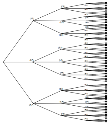
We count, after n tests, the total number of success obtained. If we denote by  this random variable then the possible values of
  are
are  . In addition, if we note
  the probability of having a success, then the random variable X follows a trinomial distribution noted
  such that :
 |
We note: 
In this case, one trial is realized. The possible outcomes to obtain are:  ,
,  or
or  . If we denote by
  the number of obtaining
  successes, then:
 |
The probabilities are thus:
 |
For  :
: 
In this case, two trials are realized. The possible outcomes to obtain are:  ,
,  ,
,  ,
,  or
or  . If we denote by
  the number of obtaining
  successes, then:
 |
The probabilities are thus:
 |
For  , we get:
 |
This article is an introduction for constructing of a new probability distribution called p-nomial distribution as a generalization of binomial distribution. The examples of application of this new probability law introduced in this research give us some ideas about its frequent meeting in practice.
| [1] | Yadolah Dodge, Statistique, disctionnaire encyclopédique, Paris 2007. | ||
| In article | |||
| [2] | Anders Hald, A History of Probability and Statistics and Their Applications before 1750, John Wiley & Sons, 2005. | ||
| In article | |||
| [3] | Eric Gossett, Discrete Mathematics with Proof, John Wiley & Sons, 2009. | ||
| In article | |||
| [4] | Michiel Hazewinkel, Encyclopaedia of Mathematics, vol. 2, Springer Science+Business Media, 1994. | ||
| In article | View Article | ||
| [5] | Norman Johnson, Adrienne Kemp and Samuel Kotz, Univariate Discrete Distributions, John Wiley & Sons, 2005 | ||
| In article | View Article | ||
| [6] | Alan Ruegg, Probabilités et statistique, vol. 3, PPUR, 1994. | ||
| In article | |||
| [7] | Aziz ATTA, “p-nomial Coefficients and p-nomial Theorem.” Turkish Journal of Analysis and Number Theory, vol. 8, no. 1 (2020): 6-15. | ||
| In article | View Article | ||
| [8] | F.M. Dekking C. Kraaikamp H.P. Lopuhaa L.E. Meester, A Modern Introduction to Probability and Statistics, Understanding Why and How, Delft Institute of Applied Mathematics Delft University of Technology Mekelweg 4 2628 CD Delft The Netherlands. | ||
| In article | |||
| [9] | Charles M. Grinstead, J. Laurie Snell, Introduction to Probability, Swarthmore College and Dartmouth College, USA. | ||
| In article | |||
| [10] | Aziz ATTA, “Twin Polynomials and Kernels Matrix.” Turkish Journal of Analysis and Number Theory, vol. 8, no. 3 (2020): 57-69. | ||
| In article | View Article | ||
| [11] | Andreas N. Philippou, Demetrios L. Antzoulakos, Binomial Distribution, Chapter · January 2011, | ||
| In article | View Article | ||
| [12] | Matthew Aldridge, Measure Theory and Integration: Measures, MA40042, UK. | ||
| In article | |||
| [13] | M. Samuel Fiorini, MATH-F-307 Mathématiques discrètes, Version du 5 octobre 2012. | ||
| In article | |||
Published with license by Science and Education Publishing, Copyright © 2020 Aziz ATTA
![]() This work is licensed under a Creative Commons Attribution 4.0 International License. To view a copy of this license, visit
http://creativecommons.org/licenses/by/4.0/
This work is licensed under a Creative Commons Attribution 4.0 International License. To view a copy of this license, visit
http://creativecommons.org/licenses/by/4.0/
| [1] | Yadolah Dodge, Statistique, disctionnaire encyclopédique, Paris 2007. | ||
| In article | |||
| [2] | Anders Hald, A History of Probability and Statistics and Their Applications before 1750, John Wiley & Sons, 2005. | ||
| In article | |||
| [3] | Eric Gossett, Discrete Mathematics with Proof, John Wiley & Sons, 2009. | ||
| In article | |||
| [4] | Michiel Hazewinkel, Encyclopaedia of Mathematics, vol. 2, Springer Science+Business Media, 1994. | ||
| In article | View Article | ||
| [5] | Norman Johnson, Adrienne Kemp and Samuel Kotz, Univariate Discrete Distributions, John Wiley & Sons, 2005 | ||
| In article | View Article | ||
| [6] | Alan Ruegg, Probabilités et statistique, vol. 3, PPUR, 1994. | ||
| In article | |||
| [7] | Aziz ATTA, “p-nomial Coefficients and p-nomial Theorem.” Turkish Journal of Analysis and Number Theory, vol. 8, no. 1 (2020): 6-15. | ||
| In article | View Article | ||
| [8] | F.M. Dekking C. Kraaikamp H.P. Lopuhaa L.E. Meester, A Modern Introduction to Probability and Statistics, Understanding Why and How, Delft Institute of Applied Mathematics Delft University of Technology Mekelweg 4 2628 CD Delft The Netherlands. | ||
| In article | |||
| [9] | Charles M. Grinstead, J. Laurie Snell, Introduction to Probability, Swarthmore College and Dartmouth College, USA. | ||
| In article | |||
| [10] | Aziz ATTA, “Twin Polynomials and Kernels Matrix.” Turkish Journal of Analysis and Number Theory, vol. 8, no. 3 (2020): 57-69. | ||
| In article | View Article | ||
| [11] | Andreas N. Philippou, Demetrios L. Antzoulakos, Binomial Distribution, Chapter · January 2011, | ||
| In article | View Article | ||
| [12] | Matthew Aldridge, Measure Theory and Integration: Measures, MA40042, UK. | ||
| In article | |||
| [13] | M. Samuel Fiorini, MATH-F-307 Mathématiques discrètes, Version du 5 octobre 2012. | ||
| In article | |||


