It is a review work, the journey being from the birth of an algebraic structure ‘Region” (the minimal but most important algebraic structure in Algebra), then to the “Theory of Objects” being a generalized concept of the Theory of Numbers, and then introducing “A-numbers”, and then an application of A-numbers to introduce “Region Geometry” and finally about “Region Calculus”. The work reports the recent developments in Pure Mathematics at its fundamental level. On making a quick visit to the notion of the minimal but most important algebraic structure Region, and then on making a quick visit to the ‘Theory of Objects”, the author here develops a new theory called by “Theory of A-numbers” corresponding to a complete region A. The classical “Number Theory” is also an instance of “Theory of A-numbers” when the complete region A is the particular complete region RR corresponding to the region R. The new notion of im-numbers and compound numbers introduced in Number Theory will play huge role in future research work in the STEM subjects. The notion of “im-number” is a generalized concept of the ‘imaginary number i’, and the notion of “compound numbers” is a generalized concept of complex numbers. And then an application of the notion of A-numbers is done to introduce a new geometry called by ‘Region Geometry’ in Pure Mathematics. Finally, a new concept of calculus is developed called by “region Calculus” in the style of Newton’s calculus. Region calculus is a unified model of all possible calculus, and Newton calculus can be viewed as a particular instance of ‘Region Calculus’. The complete work reported here launches a new topic “Region Mathematics” in the giant subject Pure Mathematics. And the work will certainly cater to the future research activities in Pure Mathematics, in all the STEM subjects, including Data Science, AI and modern Statistics.
This work is a review type work but integrating few new concepts recently introduced in the subject Pure Mathematics. In the work 1, a new algebraic structure ‘Region’ is introduced to fix a hidden serious gap in the existing giant subject Algebra. In the work 2 the author developed the “Theory of Objects” and it is justified that the “Theory of Objects” is a super concept of the classical Number theory. Theory of Objects introduces few new topics viz. prime and composite objects, imaginary and compound objects, im-numbers and compound numbers, the concept of ‘Object Linear Continuum Line’ etc in the complete region A. The notion of “im-number” is a generalized concept of the imaginary number i, and the notion of “compound numbers” is a generalized concept of the complex numbers. The notion of im-numbers and compound numbers will enrich the existing Number Theory for future applications in all the STEM subjects. In this work, the author then introduces a new theory called by “Theory of A-numbers” corresponding to a complete region A. If a region K is not a complete region, the “Theory of K-numbers” does not exist for it. Before developing the theories about A-numbers, a quick visit to the algebraic structure ‘Region’ and the main concepts about the ‘Theory of Objects’ is made for ready reference. Then an application of A-numbers is done to introduce a new kind of geometry with objects (by object we mean an element of a set 3 or multiset). Finally a generalized form of all calculus is made by introducing the notion of “Region Calculus” in Pure Mathematics.
We first of all consider the term “Key List” as below..
Consider a list of key algebraic structures in Algebra which are:-
Semi Group, Group, Ring, Integral Domain, Module, Field, Linear Space, Algebra over a field and Extensions, Associative algebra over a field, F-algebra, Division Algebras, Euclidian Hurwitz Algebra, Cayley–Dickson algebra (Octonion Algebra), Clifford Algebra, Quaternion Algebra, universal algebra, etc.
For the purpose of frequent uses of these algebraic structures in this work, let us call this list by the name “Key List”.
For details about the algebraic structures mentioned in the above Key List, and about the history of Number Theory, one could see the excellent literatures like 4, 5, 6, 7 [8-30] 8.
It is justified in length and established by several examples in 1 that the existing huge volume of algebraic structures in the subject “ALGEBRA” is incomplete to validate many elementary frequently practiced algebraic computations like: square or cube (or nth power) of an algebraic expression, frequently practiced few identities, Cross-Multiplication rule, and many more. None of the algebraic structures of the Key List (as defined above) can validate these computations by their respective definitions and by virtue of their respective properties, except the newly introduced algebraic structure ‘region’. Even an important, very useful and most frequently used Cross-Multiplication rule, which has been being used fluently by the mathematicians and by the scientists of all the STEM subjects for last several centuries, can not be validated (can not be verified) by any individual algebraic structure of the Key List. Many mathematicians of this century may summarily reject this above statement, because of the strong reason that: “How come the above fact about “Cross-Multiplication Rule” can be true which have been fluently and successfully used by all scientists for several past centuries without having any erroneous or wrong result?’. Yes, although the above statements seem to be unimaginable, impossible and very difficult to accept in mind in this century by any of the world mathematicians, but this genuine fact is revealed in 1 in details. The following examples highlight the serious structural gaps in Algebra. This serious gap in the subject Algebra has been discovered and fixed in the work 1. The minimal platform required for practicing elementary algebra is the region algebra, not any algebra member of the Key List.
An algebraist can define an infinite number of new algebraic structures. The objective behind the work 1 is not just for the sake of defining a new algebraic structure, and is not to increase the volume of literature of Algebra unnecessarily; but to recognize and identify a major gap of the giant subject ‘Algebra’ lying hidden so far in the existing vast literature of it, and then to fix the gap.
Example 2.1
Consider a very simple instance from elementary algebra, a type which is very frequently used by the secondary school students and ofcourse by the world researchers, is the equality (identity) I of following type:
 =
=  ,
,
where x, y are in an algebraic structure A (assume that the name of the algebraic structure A is not known at this moment) and a, b are two members (scalars) of some known field F.
We would like to say that this beautiful and simple identity is not valid i.e. ‘can not be verified’ in a Group, or in a Ring, Integral Domain, Field, Linear Space, in any F-Algebra, Associate Algebra, Division Algebra, Normed Division Algebra, Clifford Algebra, Cayley Algebra, Cayley–Dickson algebra or in any existing standard brand of algebraic structure alone in general (as listed in the Key List), by virtue of their respective definitions and independently owned properties.
See the justification presented below, about this simple identity I.
Justification
since division operations are involved in both LHS and RHS expressions of the identity I, the unknown algebraic structure A can not be a ‘F-algebra’ by virtue of its definition and independently owned properties.
next, if it is not a ‘F-algebra’ then let us check whether it could be a division algebra D (remembering that every field is also a division algebra).
Then the following are fact by virtue of the definition and independently owned properties of the division algebra D:-
(i) the LHS expression  of I can be well written to be equal to the expression
 (x*y-1) in the division algebra D,
(ii) but next the expression 
 (x*y-1) can’t be written to be equal to the expression (a
 x) *
x) * in the division algebra D, by virtue of the definition and own properties of “division algebra”.
[although, it is true that in the division algebra D, by virtue of its definition and owned properties, whereas the expression (a x) *
x) * can be written equal to the expression
  ].
].
Consequently, in a division algebra D, the expression  can not be accepted in general to be equal to
  , by virtue of its definition and own properties. This is a great failure of Division Algebra, whereas the identity(equality) of type I are very frequently being used by the mathematicians.
Out of all the existing recognized algebras of the Key List, none can prove (i.e none can validate) the above identity/equality I, cross-multiplication rule !! This is a serious setback of the existing volume of literature of the subject ‘Algebra’.
It has been remaining unknown so far that fortunately the set R of real numbers satisfies some additional interesting properties, which are beyond the properties of it possessed by virtue of the definition and properties of the algebraic structure ‘division algebra’ or by any algebraic structure so far developed in the subject Algebra. And that is the hidden reason why the mathematics has not been facing any problem and have not been getting any incorrect final results or contradictory results in R, while applying the above type of identities I in mathematics, exercises and computations in science subjects or engineering subjects or in any STEAM subject. The situation is equivalent to driving a car for past centuries on the roads by a driver without having a valid driving license from any authority, without any accident!!.
Example 2.2
With exactly the same argument as in Example 2.1 above, it can be observed that if an algebraic equality (in fact it is an identity) J of type given by

happens to be a valid identity (i.e. can be computed and verified) in an algebraic structure A where x, y  A, a and b being members (scalars) of some given field F, then it can be observed that each of the following five statements are true:-
(a) A is not a group, or a ring, or integral domain or module, field, linear space, etc by virtue of their respective definitions and independently owned properties.
(b) A is not an ‘algebra over a field F’ (F-algebra) by virtue of its definition and independently owned properties.
(c) A is not an ‘associative algebra over a field’ by virtue of its definition and independently owned properties.
(d) A is not a ‘Division Algebra’ by virtue of its definition and independently owned properties.
(e). A is not any standard existing brand of algebraic structure or of any standard extension, by virtue of its definition and independently owned properties.
Undoubtedly, if the above identity named by J (and also the identities of Example 2.1) can not be validated by any existing algebraic structure A or existing extensions, then our giant subject “Algebra” must identify: “Who is this unknown algebraic structure A in whom these identities are valid by virtue of their respective definition and independently owned properties?” Otherwise the subject Algebra will remain as a subject having few serious gaps. Consider now a very important and interesting example below.
Example 2.3
It is known that the following computation is known as ‘Cross-Multiplication’ rule C of elementary algebra :
if  =
= 
then (a.d) x
x t = (b.c)
 y
y z(and conversely),
where x, y, z, t are in an algebraic structure A (the name of this algebraic structure A is not known at this moment) and a, b, c, d are the members (scalars) of some given known field F. Then C ‘can not be verified’ (i.e. can not be validated) in general in any algebraic structure of the Key List, just by virtue of their respective definitions and independently owned properties. The justification in brief regarding this very popular ‘Cross-Multiplication’ property C is presented below:-
Justification:
The justification is in fact similar to what made in the case of Example 2.1 above.
Since division operations are involved in both LHS and RHS expressions, A can not be a ‘F-algebra’ by virtue of its definition and independently owned properties.
In the next step, since it is not a ‘F-algebra’, then let us check whether it could be a division algebra D (remembering that every field is also a division algebra). Then the following are fact by virtue of the definition and independently owned properties of division algebra:-
Suppose that the given equality  =
=  being considered here is in the algebraic structure A which is a “division algebra”. Then, from this equality, we arrive at the very next equality which is

 =
= 
 valid in the division algebra A. Upto this point, there is no issue.
But after this step, the existing Algebra gets blocked and can not proceed further for any next further step in the division algebra A. Because this can not yield the next step of the computation expected (and required by us) to be as below
(a.d) x
x t = (b.c)
 y
y z
z
in the division algebra A just by virtue of its definition and its independently owned properties of the algebraic structure ‘division algebra’. Recollect that ‘Compatibility with the scalars of the field F’ does not hold good in a division algebra A in general.
Example 2.4
It can also be seen that this type of simple square identity I like:
 =
=  ( where c = a2 and d = b2)
(where x, y, z, t are in an algebraic structure A (the name not known at this moment, what is the name of this algebraic structure) and a, b, c, d are members (scalars) of some field F) ‘can not be verified’ (i.e. can not be validated) in general in any algebraic structure of the Key List, just by virtue of their respective definitions and independently owned properties. Then, the immediate questions that arose in mind are:-
• “What is the minimal algebraic structure which can validate the above examples?” Or
• “What could be the minimal algebraic structure in which the above type of identities like I or the above type of cross multiplication results like C, etc are valid?”. Or
• “In what minimal algebraic structure, the above type of identities like I or the above type of cross multiplication results like C, etc can be verified?”.
Note carefully that, in the above four examples we are talking about identities, square of an algebraic term, cross-multiplication rule etc which are being very frequently used and very importantly used in computations by the students and researchers in mathematics, statistics, science subjects, engineering subjects etc since past centuries.
An algebraist can not answer what is this unknown algebraic structure A in the above four examples. He must answer a unique name of an algebraic structure, because of the reason that these type of examples are of tremendous practices by the students and mathematicians in their daily computational works and activities. Is it a Group?, or Ring? or Integral Domain, Field, Extension of Field?, or Linear Space, F-Algebra, Associate Algebra, Division Algebra, Normed Division Algebra, Clifford Algebra, Cayley Algebra, Cayley–Dickson algebra or any standard algebraic structure (assuming that division by zero element is not allowed), etc??. For a possible answer, because of non-availability from the existing huge volume of algebraic structures of the subject ‘Algebra’, the algebraist has to think of a permutation/combination of the various existing algebraic structures (and their extensions) to discover a possible result. But, he might seek to make a unique identity for this algebraic structure A (a minimal algebraic structure A) to define it in an independent and atomic way, as the algebraists did the same earlier too to define ring, field, division algebra, ... etc instead of “not doing” and managing by the-then existing algebraic structures by exercising their permutation/combinations; because ‘Algebra’ must be sound and complete in this sense. Consequently there a genuine need to identify this minimal algebraic structure, which is hidden so far, un-discovered far, for practicing the elementary algebra and higher algebra more appropriately. Truly speaking, ‘Region’ is the most practiced algebra in school/college education, research, scientific and engineering calculations, etc in a hidden way. In the work 1, it is established that ‘Region’ is the minimal algebra to study science, mathematics, engineering, and other areas. None of the existing algebraic structure has this capability. A quick visit to the definition of Region is presented below:-
2.1. The ‘Minimal’ and ‘Most Useful’ Algebraic Structure in the Subject AlgebraIt is very important to note the word minimal used here, corresponding to the new algebraic structure “Region”.
REGION
Consider a non-null set A with three binary operators  ,
,  and
and  defined over it such that for a given field (F, +, .), the following fourteen(14) conditions are satisfied:-
(A,  ) is an abelian Group with respect to addition:
(1) if x, y, z  A then (x
 y)
y) z = x
z = x (y
(y z).
z).
(2)  0A
0A  A such that x
 0A = x = 0A
 x,
x,  x
x A.
A.
(3) if x A,
A,  y
y A such that x
 y = 0A = y
 x.
x.
(4)  x, y
x, y A, x
A, x y = y
y = y x.
x.
(A, *) forms an Abelian Group (excluding the element 0A) with respect to multiplication:
(5) if x, y, z  A then (x
 y)
y) z = x
z = x (y
(y z).
z).
(6)  1A
1A  A such that x
 1A = x = 1A
 x,
x,  x
x A.
A.
(7) if x  A,
A,  y
y A such that x
 y = 1A = y
 x.
x.
(8)  x, y
x, y  A, x
A, x y = y
y = y x.
x.
Distributive Properties:
(9)  x, y, z
  A,
A,
(i) x (y
(y z) = (x
 y)
y) (x
(x z).
z).
(ii) (x y)
y) z = (x
 z)
z) ( y
( y z).
z).
Scalar Multiplication:
(10) Scalar multiplication of x A by element k
 F, denoted by k
 x is to be in A,
(11) k (m
(m x) = (k.m)
 x, where x
 A, and k, m
  F.
F.
(12) k (x
(x  y) = k
 x
x  k
k y,
y,
where x, y A, and k, m
 F.
F.
(13) (k + m) x = k
x = k x
x  m
m x,
x,
where x A, and k, m
  F.
F.
Compatibility with the scalars of the field F:
(14) A satisfies the property of “Compatibility with the scalars of the field F”,
i.e. (k x ) * (m
 y ) = (k.m)
  (x*y)
(x*y)
 k, m
k, m  F and
F and  x, y
x, y  A.
A.
Then the algebraic structure (A,  , *,
, *,  ) is called a Region over the field (F, +, .).
If there is no confusion, we may simply use the notation A to represent the region (A,  , *,
, *,  ), for brevity. It may be observed that if (A,
  , *,
, *,  ) be a Region over the field (F, +, .), then (A,
  , *) is a field and (A,
  ,
,  ) is a linear space over the field (F, +, .). However, being a field as well as a linear space does not suffice to become a region. The above definition of region may be presented alternatively as below:-
Consider a non-null set A with three binary operators  , * and
  defined over it such that for a given field (F, +, .), the following three(3) conditions are satisfied:-
(i) (A,  , *) forms a field,
(ii) (A,  ,
,  ) forms a linear space over the field (F, +, .), and
(iii) A satisfies the property of “Compatibility with the
scalars of the field F”,
i.e. (k x ) * (m
  y ) = (k.m)
 (x*y)
(x*y)
 k, m
k, m  F and
F and  x, y
x, y  A.
A.
Clearly a region is not just a division algebra only, but having a lot of amounts of more mathematics in it. A division algebra, in general, is not a region. However, one could try to view a region by permutation/combination of some of the existing classical algebraic structures in other ways. For instance, the following two theorems follow directly from the axioms (definition).
Theorem 2.1
Let (A,  , *, ·) be a Region over a field F. Then the following are true:
(i) (A,  , *) is a commutative field,
(ii) (A,  , ·) is a vector space over F,
(iii) (k·x) *(m·y) = (km)·(x*y).
Theorem 2.2
Every Region is a commutative division F-algebra.
Consider the following interesting simple problem on Algebraic Computations.
Problem 2.1.
Obtain an expression for x in terms of y and t from the following equation in the real region (A, ,
, ,
, ):
):
3 x* y = 2
 y
y 3
3 t ,
t ,
where x , y ( 0A), t
  A.
A.
Solution:
We have the following equation in the region A:
3 x * y = 2
 y
y 3
3 t
t
Using the properties of region, we then can write

 (3
(3 x*y) =
 (2
(2 y
y  3
3 t )
t )
or, 
 (x*y) =


or, 1F (x*y) =
 y
y 

 t
t
or, x*y = 
 y
y 1F
1F  t
t
or, x*y = 
 y
y t
t
or, ( x*y )*y -1 =  *y -1
*y -1
or, x * ( y * y -1 ) = 
 ( t * y -1 )
or, x*1A = 
 ( t * y -1 )
or, x =  , which is the solution.
An Interesting Analysis about the above ‘solution’ :-
Let us analyze now the solution to the above Problem 2.1. For this, we begin our analysis with an element of imagination equipped with the following two points:-
Point (i): It is already given in the problem statement that the algebraic structure A is a region. But, let us imagine a situation that the identity of the algebraic structure A in the above Problem 2.1 is “unknown” to us at this moment, and we are dealing with the existing Algebra only. And also let us accept that
Point (ii): let us also accept that the solution steps presented above are well valid and correct in this “unknown” algebraic structure A.
Now, in the above solution steps, we see that:-
there are few steps (not all the steps) which are allowed by virtue of the definition and properties of ‘vector space’, and there are few steps (not all the steps) which are allowed by virtue of the definition and properties of ‘division algebra’. It may be carefully observed that a ‘division algebra’ can not give license to all the steps of the above mentioned solution-method by virtue of its own definition and independently owned properties (for example, ‘compatibility with scalars’ is not a licensed step in division algebra, even not the commutative property).
Besides that, see that division operations are executed in the solution steps. Hence A can neither be just an ‘algebra over a field’ nor an ‘associative algebra over a field’.
Consequently, considering the validity of “all the involved operations collectively” in the steps of the above mentioned solution-method, it is now obvious that this unknown algebraic structure A of this Problem 2.1 has to be at minimum a ‘region’, not less (i.e. not a Division Algebra, not any of the existing standard algebraic structures listed in the Key List). The above simple example of solution-methods (as this problem can not be solved for x in any of the algebraic structure mentioned in the Key-List) shows that there is a serious gap in the existing “ALGEBRA”. There must be a unique identity of this unknown algebraic structure A, because the existing subject Algebra (with all its existing algebraic structures and extensions) fails by its existing vast rich literature to solve the above Problem 2.1 !!! And now it can be seen that this unique minimal algebra A is “Region”, not any algebraic structure mentioned in the Key List..
In this section, we do more amount of characterizations about the minimal algebraic structure region. In our work here, we use the following notations fluently:
R = set of all real numbers, R+ = set of all positive real numbers, R- = set of all negative real numbers, R≥0 = set of all non-negative real numbers.
Let R be the set of real numbers, ‘+’ be the ordinary addition operator in R and ‘.’ be the ordinary multiplication operator in R. Consider the field ( R,+, . ) of real numbers, and the linear space (R,+, .) over the field (R,+, .) . Then the algebraic system (R,+, . , .) forms a region over the outer field (R,+ , .).
This region (R,+ , . , .) plays a very important role in our daily life computations, in particular in school level elementary algebra. The content of the syllabus and corresponding instructions at school level algebra is based on the platform of this region (R,+, . , .), not on the platform of any standard algebraic structure like groups, rings, integral domains, fields, linear spaces, algebra over a field, associative algebra over a field, division algebra or any existing algebraic structure. Let us name this region (R,+, . , .) in short by the word “RR”. The region RR is the most useful region in all the branches of Mathematics, Statistics, Science, Engineering etc i.e. in all STEM subjects.
The very interesting properties of the region RR are :
(i) its inner field is (R,+, .),
(ii) its outer field is also (R,+, .),
(iii) all the three multiplication operators are same, and
(iv) all the three addition operators are same.
2.2. Real RegionA region (A,  , *,
, *, ) over the field ( F, +, . ), is called a Real Region if its outer field F is the classical field R of real numbers.
Example 2.2.1
The regions RR, C are examples of real region.
In Region Algebra, the characteristic of a region A denoted char(A) is defined to be the smallest number of times one must use its multiplicative identity 1A in a sum to get the additive identity element 0A. A region is said to have characteristic zero if this sum never reaches the additive identity. For example, for the region RR we have Char(RR) = 0.
2.3. Partitioned RegionConsider a real region A = (A, ,*,
,*, ). Suppose that A forms a chain with respect to a total order relation (say, denoted by the notation ‘
 ’). Then the real region A is called a chain region with respect to the total order relation ‘
 ’.
’.
A real region A = (A, ,*,
,*, ) is called a Partitioned Region if the following conditions are satisfied:
(i) A is an infinite region,
(ii) A is a chain region with respect to a total order relation
‘ ’, and
(iii) the characteristic of A is zero.
Here A is called a ‘partitioned’ region because of the fact that it induces a partition PA of the region A into three mutually disjoint non-null sets denoted by A+, A- and {0A} such that
(i) A+ = { a: a A and 0A < a}
(ii) A- = { a: a  A and a < 0A}.
Clearly,  a
a  A+, ~a
  A- and
  b
b  A-, ~b
  A+.
A+.
(Note: It may be recalled from the properties of the chain that: a < b iff a ≤ b and a ≠ b, where “≤” is the total order relation of the chain A, and similarly a > b iff b ≤ a and b ≠ a).
The partition PA, once made, is regarded as an absolute partition of the region A corresponding to its total order relation ‘ ’ in the sense that this partition generates the sign of every object of the complete region A, positive or negative, which will remain absolute throughout the complete literature henceforth . However for a different type of total order relation defined over the region A we will get a different partition of A. But the set {0A} is common to all such possible partitions of A.
Consider an infinite region A = (A, ,*,
,*, ). The extended region of the region A is the region itself with all its infinity objects, if any. The infinity objects are not basically the core member of the region A. For the RR region and the C region, the concept of infinity is known to us. Infinity is not an element of the set R of real numbers. Instead, the real line extends infinitely in both the directions, leading to positive infinity (+
 ) and negative infinity (-
 ) which are included in the extended real number system, but not included in R. An analogous concept gives the notion of Complex infinity. It is like a complex number ( 7, 22) with infinite magnitude and an undefined argument. The most common representation is Riemann Sphere where all infinite paths are wrapped around a sphere. At this point of time we do not consider any method about ‘how to find out all the infinity objects of an infinite region’. Even for the present work, we do not need to study the existing advanced theories of infinities so far developed in Mathematics. However for a partitioned region the method is rather easier about considering the concept of infinity as mentioned below, and in this work all-through, whenever the notion of infinity is to be used, we must consider only those regions which are partitioned regions.
Consider a partitioned region A = (A, ,*,
,*, ). If we now include two more objects +
 A and -
 A in A as two permanent guests, then the set AE = A
  {+
{+ A, -
A, - A} is the ‘extended region’ of the region A.
The two guest objects + A and -
 A are called infinities, and are defined as below:
(i) + A =
A =  where
where  (≠ 0A) is any positive object of the partitioned region A, and
(ii) - A =
A =  where
where  (≠ 0A) is any negative object of the partitioned region A.
The extended region of the partitioned region A is denoted by the notation AE. However, if there is no confusion then we may use the notation A itself to denote the extended region of A. Note that an extended region is not a region. For a partitioned region, it is just a superset of the set A containing two more objects.
But whenever we say that ‘A is an extended region’, it will simply mean that A is a region with all its infinities as permanent guests. At this stage we do not explore to study whether there are more infinities other than the two guest objects + A and -
 A for a partitioned region.
An extended region AE may be called as ‘extended real region’ if the corresponding region A is a real region.
For the region C, there are many infinities to be included into it to call it an extended region. For example  a, b
a, b  R, the object a+ib is an infinity object for C if either a or b or both are the infinity object of the region R. The extended region of C is denoted by the notation CE. Further future study on the topic of extended region will make the literature richer. However, in our work here we use the case of the extended region of a partitioned region only.
A quick visit to the algebraic structure ‘Region’ is made in Section-2. To introduce the Theory of A-numbers, as a pre-requirement, we need to pay a quick visit to some portions of the work 2 too, as presented below. The notion of im-number is a generalized concept of imaginary number, and the notion of compound numbers is a generalized concept of the complex numbers. For details about the notion of im-numbers and compound numbers introduced in Number Theory, one could see 2. The notion of compound number introduced in 2 is a revised version of the same introduced in 31.
3.1. 2-to-1 Bijective MappingConsider two non-null sets X and Y. A function
f : X  Y is said to be a ‘2-to-1 Bijective Mapping’ if
(i) f is onto, and
(ii)  y
y Y,
Y,  two and only two distinct (not same)
elements x1 and x2 in X such that f(x1) = y = f(x2).
For example, the function f: R-{0} R+ given by f(x) = x2 is a 2-to-1 Bijective Mapping.
But the function g: R R+ given by g(x) = x2 is not a 2-to-1 Bijective Mapping.
Consider a partitioned region A = (A, ,*,
,*, ) with respect to the total order relation ‘
 ’. Then A forms a Region Space if the following conditions are satisfied:
(i) A is an extended region
(i.e. A is a region and two infinities are also
included to it as permanent guests).
(ii) A is a normed complete metric space with respect to a
norm ║.║ and the corresponding induced metric
ρ(x, y) = ║x~y║, (i.e. ║x║ = ρ(x, 0A) ).
(iii) The norm ║.║ is a 2-to-1 bijective mapping from
A – {0A} to R+.
3.3. Complete RegionA real region which forms a region space is called a “complete region”.
We will introduce here later that by a complete region, we will always mean one-dimensional complete region (1-D complete region). For instance, the region RR is a complete region with respect to the crisp order relation “Less Than or Equal To” denoted by the notation “≤” and the metric ρ(x, y) = ║x - y║ = |x-y|, where the norm is the classical norm defined over R. The collection of all the complete regions is called the complete region universe Ʃ.
3.4. Positive Object and Negative ObjectConsider a partitioned complete region A = (A, ,*,
,*, ). The three sets of the partition of a region are denoted by A+, A- and {0A} where A is a chain region with respect to a total order relation ‘
 ’.
’.
The elements of A+ are said to be positive objects and the elements of A- are said to be negative objects. The object 0A is neither in A+ nor in A-, and so we say that the object 0A is neither a positive object nor a negative object. The attribute of being positive or negative is called the sign of the object, and the object 0A is not considered to have a sign of its own.
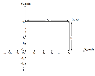
3.5. Object Linear Continuum LineA line can be drawn on plain paper on which one point may be fixed to be the location for the zero object 0A, with all positive objects of A having their respective locations to the right and all negative objects of A having their respective locations to the left of the zero object 0A. The term ‘location’ will be more clear soon. Thus the ‘positive direction’ of the line can be called to be XA-axis and the ‘negative direction’ of the line can be called to be XA1-axis. And the line which the objects of the complete region A is considered to lie upon is called the Object Linear Continuum Line for the complete region A (see Figure 3.1).

Thus, any point on the Object Linear Continuum Line of the complete region A is called an object point of A.
For developing a Object Line over a region A, it must be a region space. Consider the object linear continuum line and the corresponding XA-axis. Since the region A is complete, there are no "points missing" from it (inside or at the boundary). Since A is a chain, every object of A has a unique address on this object linear continuum line and conversely i.e. corresponding to every address (point) on this ‘object linear continuum line’ (see Figure 3.1) there is a unique object of the region A. This property is called “Completeness Property” of this complete region A.
Consider a point x on the X-axis of the object linear continuum line corresponding to the region space A. Then for an infinitesimal small positive object ∆x of the region A, the point (x ∆x) will be at a distance ║∆x║ from the point x along the positive direction of X-axis and the point (x ~ ∆x) will be at a distance ║∆x║ from the point x along the negative direction of X-axis. By distance between two objects x and y lying upon the XX1 Object Linear Continuum Line of the complete region A, we mean the corresponding metric distance ρ(x,y) of the normed complete metric space A.
The distance of a positive object xA from the origin is  = ρ(xA, 0A) = xa, and consequently the distance of a negative object ~xA from the origin is -xa (on imposing minus sign for convention). For example, see a collection of consecutive equi-spaced points on the object line as shown in the Figure 3.2 below.

The term ‘equi-spaced’ in the caption of Figure 3.2 is well understood in the sense of the corresponding metric (or norm) of the complete region A,
i.e. for any real integer r,
ρ(r 1A, (r+1)
 1A) = constant (independent of r), in the complete region A by virtue of the beautiful property of ‘Homogeneity’ possessed by the metric ρ.
The following theorems follow directly from the above constructions:-
Theorem 3.1
(i) For every positive object x of the region space A,
x = ║ x ║ 1A
1A
(ii) For every negative object x of the region space A,
x = ~║ x ║ 1A
1A
Theorem 3.2
The unit element 1A of the region space A is at the distance 1 (real integer) on the right side of the zero element 0A on the object linear continuum line of A.
Theorem 3.3
The positive object x of the region space A is located at a distance ║ x ║ from the zero element 0A on the right side of 0A on the object linear continuum line, and the negative object x is located at a distance ║ x ║ from the zero element 0A on the left side of 0A,
Since A = (A, ,*,
,*, ) is a complete (normed complete metric space), there are no "points missing" from it (inside or at the boundary). Since A is a chain, every object of A has a unique address on this Object Linear Continuum Line XA1XA; and conversely i.e. corresponding to every address (point) on this Object Linear Continuum Line XA1XA there is a unique object of the region A.
Example 3.1
If we choose the region A to be the RR region (see Example 2.4 presented earlier) which is a partitioned region with respect to the crisp order relation “Less Than or Equal To” denoted by the notation “≤”, and if we choose ║x║ = |x| in RR, where ρ(x, y) =║x-y║= |x-y|, then it can be observed that the X-axis of the region calculus is the classical X-axis popularly used by us in the Cartesian coordinate system in Geometry.
In this section the “Theory of A-numbers” is introduced, by defining the concept of onteger. For an history about numbers, one could see 32, 33, 34. First of all we define Unit Length on the object linear continuum line XA1XA.
4.1. Unit LengthWe define now the concept of ‘Unit Length’ in a complete region A. Consider a complete region A = (A, ,*,
,*, ). If xA is a positive object on the object linear continuum line, then the distance of the point xA from the point O (the location of the object 0A on the object linear continuum line XA1XA) is a positive real number denoted by the notation xa . We use the traditional practiced convention to say that ~xA is at a distance of –xa (imposing minus sign) from the point O, although as per definition of metric a distance can not be a negative quantity.
For xA  A, we have
 = xa , if xA is a positive object,
= - xa , if xA is a negative object
because ρ(0A, xA) = ρ(0A, ~xA) =  .
.
Corresponding to the unit element 1A of the complete region A, the positive real number 1a (where 1a = ║1A║ = ρ(0A,1A)) is called the ‘unit length’ in the Theory of A-numbers. Thus the “unit length” is defined by the distance of the object 1A from 0A. Clearly 0a being the ║0A║ is equal to the real number 0.
Proposition 4.1
For every complete region A, the value of its “unit length” is equal to 1.
Proof. Straightforward from the axiom of the normed linear space.
From the identity ║1a 1A║ = ║1A║,
we have |1a|.║1A║ = ║1A║.
Therefore, |1a| = 1, i.e. 1a = 1. Hence proved.
4.2. Ontegers in a Complete RegionIn this section we introduce the notion of ‘Onteger’ in a complete region A = (A, ,*,
,*, ). The word ‘onteger’ is not a valid word in English dictionary. It is an abbreviated word for “Object Integer”. The concept of ‘ontegers’ will be the basic element in developing the new number theory entitled ‘Theory of A-numbers’.
Consider an object xA in the complete region A.
Therefore xA =  , ║xA║ = xa where xA is a positive object. And ~xA =
  , ║~xA║ = xa where ~xA is a negative object;.
If m is any real integer, then the object mA of the complete region A is called an ‘object integer’ or ‘onteger’ in the ‘Theory of A-numbers’.
Thus the ontegers in the ‘Theory of A-numbers’ are 0A,  1A, ~1A,
  2A, ~2A,
  3A, ~3A, ….. etc. The ontegers
  1A,
1A,  2A,
2A,  3A,
3A,  4A, …….. etc. are ‘positive ontegers’ and the ontegers ~1A, ~2A, ~3A, ~4A, …….. etc. are ‘negative ontegers’ in the ‘Theory of A-numbers’. The onteger 0A is neither a positive onteger nor a negative onteger. Obviously, the set of all ontegers of the complete region A is a countable set. However, it may be true that norm of some of the ontegers of the complete region A are integers in R. In a complete region A, the ontegers 0A,
  2A, ~2A,
  4A, ~4A, ….. are even ontegers and the ontegers
  1A, ~1A,
  3A, ~3A
  5A, ~5A …….. are odd ontegers. For a given complete region A the distance between two consecutive ontegers on the object linear continuum line will be always a constant real number. Thus, we have for the complete region A,
…… = ρ(~3A, ~2A) = ρ(~2A, ~1A) = ρ(~1A, 0A) = 1 = ρ(0A, 1A) = ρ(1A, 2A) = ρ(2A, 3A) = ρ(3A, 4A) = …… ,
and similarly for the complete region B,
…… = ρ1(~3B, ~2B) = ρ1 (~2B, ~1B) = ρ1(~1B, 0B) = 1 = ρ1(0B, 1B) = ρ1(1B, 2B) = ρ1(2B, 3B) = ρ1(3B, 4B) = ………. . For any real number r, ρ(r 1A, (r+1)
 1A) = positive constant 1, which is independent of the real number r. For any two real numbers r and k, we haveρ(r
 1A, (r+k)
 1A) = |k|.1 .
For an example, the ontegers of the region R are the integers (the classical notion in R).
4.3. ‘RA value’ of a Real Number x Corresponding to the Complete Region ALet A be a complete region. Corresponding to the complete region A, consider the 1-to-1 mapping
RA : R → R defined by
RA(x) = x.1a = xa  x
x  R.
R.
Then the real number xa is called the ‘RA value’ of the real number x denoted by RA(x) = xa corresponding to the complete region A.
Clearly, in that case RA(-x) = -xa. Also RA(0) = 0a = 0, and RA(1) = 1a = 1.
For xA  A, we have
 =
= 
= 
because ρ(0A, xA) = ρ(0A,~xA) =  .
.
Consider the above defined 1-to-1 mapping RRR : R → R for the complete region RR. It is obvious that RRR : R → R is an identity mapping.
4.4. ‘Natural A-ontegers’In the Theory of A-numbers, the positive ontegers  1A,
1A,  2A,
2A,  3A,
3A,  4A, … are called the ‘Natural A-ontegers’.
Proposition 4.2
Every complete region has at least one imaginary object.
Proof. Consider any complete region A = (A, ,*,
,*, ). By definition of complete region, its characteristic is zero. In our literature, by complete region we mean 1-D region calculus. We take help of an example here. Consider the
equation 
We will show that the
equation  is not satisfied by any object of A, where both LHS and RHS of this equation are “valid expressions” in A satisfying the necessary ‘qualification conditions’ as mentioned in the work 2.
Let us prove it by contradiction.
i.e. if possible, suppose that for an object xA of A we have

Or, 
Or, 
Or, 
Therefore, there is no real object xA of the region A which can satisfy the equation

Consequently, it produces one imaginary object of the complete region A which is ƐA (say). Hence the result.
(Note: It may be noted that the equation produces different imaginary objects for different complete region A. It may also be noted that although C does not form an 1-D region calculus (i.e. 1-D complete region), but it does not mean that C will not have any imaginary object.)
Proposition 4.3
(i) xa ya = (x
 y)a
y)a
(ii) (xa)n = (xn)a where n is an integer.
(iii) xA yA = (x+y)A
(iv) xA ~ yA = (x-y)A
(v) (xA)n = (xn)A where n is an integer.
Proposition 4.4
If A is a complete region, then  infinite set of trio
x, y, z  A such that the relation
is satisfied for n = 2.
Proof. Take the case for x =  , y =
, y =  and z =
  .
.
Now,  = (
= (
 )2
)2  (
(
 )2
)2
= ( )2
)2  (
( )2
)2  (
( )2
)2  (
( )2
)2
= 


= 

= (
 )2
)2
= 
This particular result can be used to generate infinite number of similar but distinct results. Hence proved.
4.5. ƐA-Complex ObjectsConsider any region A = (A, ,*,
,*, ). Since it is a complete region, by definition its characteristic is zero. As per Proposition 4.2, every such region has at least one imaginary object; this is an important result because existence of any new such imaginary object leads to a new object algebra. Consider any imaginary object of A, which is ƐA (say).
Then  the object
 is called an “ƐA-Complex Objects” corresponding to the region A. In that case the object xA is called the ‘real part’ and the object yA is called the ‘imaginary part’ of the ƐA-Complex object. Obviously both real part and imaginary part of an ƐA-Complex object are real objects of the region A.
The Ɛ-Complex Object is in fact a particular case of ƐA-Complex objects. Consider the infinite region A = (A, ,*,
,*, ) whose characteristic is zero. It is shown that the equation
  is not satisfied by any object of A. Suppose that the corresponding particular imaginary object ƐA is denoted by another notation Ɛ. Thus we have the result
  i.e. Ɛ2 = ~1A.
Then  , the object
  is called an Ɛ-Complex Object corresponding to the region A.
The set CA = { =
=  :
:  } is called the set of all Ɛ-Complex Objects corresponding to the region A.
(There should not be any confusion between the two notations CA and cA. In the Theory of A-numbers, cA is an object of the region A where CA is the set of all Ɛ-Complex Objects corresponding to the region A).
In this section a new type of algebra is developed called by ‘Algebra of Ɛ-Complex Object’. Consider the set CA of all Ɛ-Complex Objects corresponding to the region A. Denote the Ɛ-Complex Object  by the notation Ɛ0 and the Ɛ-Complex Object
  by the notation Ɛ1.
If  =
=  be an Ɛ-complex object, then we define its conjugate Ɛ-complex object given by
 =
=  .
.
Define the following operations over the set CA corresponding to the region A = (A, ,*,
,*, ). If there is no confusion, let us use the same notations
  and * of A for the case of the set CA too (although their definitions are different in A and CA).
(1) Addition & Subtraction
If  =
=  and
and  =
=  be two Ɛ-complex objects, then define addition of them using the identical notation
  as below:


 =
= 

 =
= 
which clearly belongs to CA;
and define subtraction as below:
 ~
~ =
=  ~
~ =
= 
which clearly belongs to CA.
(2) Multiplication
If  =
=  and
and  =
=  be two Ɛ-complex objects, then define multiplication of them using the identical notation
  as below


 =
= 

 =
=
 which clearly belongs to CA.
(3) Scalar Multiplication
If  =
=  and
and  =
=  be
be
Proof : Straightforward (can be proved using algebraic forms or using their norms, as seen in case of two complex numbers).
It may be observed that the set CA forms a group with respect to the binary operation  , and the set CA – {Ɛ0} forms a group with respect to the binary operation *.
Several other algebraic properties of CA can be studied in our future work.
In the work 2, a new theory titled “Theory of Objects” is developed, and it is shown that the classical Number Theory is a special case of the Theory of Objects. The notion of im-numbers and compound numbers introduced in Number Theory will play huge role in application areas in all the STEM subjects. We are now in a position to initiate a new kind of geometry on a complete region A. The “Theory of Objects” induces a new area which we call by ‘Region Geometry’ in a complete region. We begin the subject by introducing first of all a 2-D Region Geometry developed over an 1-D complete region. The new subject “Region Geometry” introduced here is in a baby stage today, but will surely take its volume soon in Pure Mathematics.
For developing the new geometry called by “Region Geometry”, be it in a two dimensional region coordinate system or in an n-dimensional region coordinate system, at least one 1-D complete region A = (A, ,*,
,*, ) is required. The work in fact is sequel to the works 1, 2.
R is a trivial example of region. And it is explained that all the materials on the subject Geometry studied in school mathematics are based upon this region R. Subject to fulfilment of some conditions, a region A opens a new Geometry. Consequently, on the platform of the region R, the classical concepts of number line, coordinate plane, x-axis, y-axis, quadrants, x-coordinate of a point, y-coordinate of a point, location of a point on the coordinate plane, line segment AB, ray, line, etc are respectively termed as number line in the region R, coordinate plane in the region , xR-axis, yR-axis, quadrants, xR-coordinate of a point, yR-coordinate of a point, location of an object point on the R-coordinate plane, line segment AB in the R-coordinate plane, ray, line etc. The work in this work is done with respect to any region A, not just with respect to a particular region R. Every region A generates its own region geometry called by ‘A-Region Geometry’ subject to fulfilment of few conditions.
Consider the object linear continuum line and the XA-axis corresponding to the complete region A. Consider a point xA (a positive object) on the XA-axis. Then for an infinitesimal small positive object ∆xA, the point (xA ∆xA) will be at a distance ║∆xA║ from the point xA along the positive direction of XA-axis and the point (xA
 ∆xA) will be at a distance ║∆xA║ from the point xA along the negative direction XA1-axis; and in fact all the objects of the complete region A are well ordered in this sense, as explained earlier. In this section we incorporate “YA-axis” (imagine that a copy of XA-axis is placed at right angle to the XA-axis passing through the point 0A, i.e. rotating through 900 anticlockwise about the point 0A) and thus construct a region coordinate plane in the style of Cartesian coordinate system.
Every complete region has its own Region Geometry. We introduce first of all 2-D Region Geometry in a 1-D complete region A = (A, ,*,
,*, ). It is a system of geometry where the position of points on the plane is described using an ordered pair of objects, analogous to the case of Cartesian coordinate plane. We call this plane by ‘Region Coordinate Plane’. A plane is a flat surface that goes on forever in both directions. If we were to place a point on the plane, region coordinate geometry gives us a way to describe exactly where it is by using two objects. Points are placed on the "region coordinate plane" as shown below in Figure 5.1. It has two scales: one running across the plane called the "XA-axis" and another at right angles to it called the “YA-axis”.
Both these axes are thus object linear continuum lines corresponding to the complete region A. The point where the two axes cross is called the origin denoted by OA at which both xA and yA are 0A. On the XA-axis, as explained earlier that objects to the right of origin are positive objects and those to the left are negative objects of A. Similarly, on the YA-axis, objects above the origin are positive objects and those below the origin are negative objects of A.
A point's location on the region coordinate plane is given by two objects in the form of object coordinates (xA, yA), the first coordinate reveals where it is away from the YA-axis at parallel to the XA-axis and the second coordinate reveals where it is away from the XA-axis at parallel to the YA-axis (see Figure 5.1 above). There are four quadrants and sign convention rule is same as that of classical Cartesian coordinate geometry. If there is no confusion, we use the word X-axis instead of XA-axis, Y-axis instead of YA-axis in our literature here.
Consider the Region Geometry corresponding to the 1-D complete region A. Consider also the Region Geometry corresponding to the 1-D complete region RR. Thus there are two sets of Region Geometry we will consider now. Suppose that the region coordinate plane of A does also represent the region coordinate plane of RR taking same lines as two axes and taking the same location for origin (i.e. OA and ORR are co-incident points). Thus the X-axis, Y-axis, and the origin are common to both the region coordinate planes.

The results of the following proposition are straightforward.
Proposition 5.1
(1)If P be a point on the X-axis with the coordinates (xA, 0A) on the region coordinate plane of A, then the coordinates of the same point P in the region coordinate plane of RR will be
(i) ( ,0) on X-axis, if xA is a positive object,
(ii) (- ,0) on X-axis, if xA is a negative object.
(i.e. the sign retaining rule will be followed, as the point P will remain in the same quadrant in both the region coordinate planes).
(2)If P be a point on the X-axis with coordinates (x, 0) on the region coordinate plane of RR, then the coordinates of the same point P in the region coordinate plane of A will be (xA, 0A) on the X-axis.
(the sign retaining rule will be followed, as the point P will remain in the same quadrant in both the region coordinate planes).
(3)If P be a point on the Y-axis with coordinates (0A, yA) on the region coordinate plane of A, then the coordinates of the same point P in the region coordinate plane of RR will be
(i) (0,  ) on Y-axis, if yA is a positive object,
(ii) (0, - ) on Y-axis, if yA is a negative object.
(the sign retaining rule will be followed, as the point P will remain in the same quadrant in both the region coordinate planes).
(4)If P be a point on the Y-axis with coordinates (0, y) on the region coordinate plane of RR, then the coordinates of the same point P in the region coordinate plane of A will be (0A, yA) on the Y-axis.
(the sign retaining rule will be followed, as the point P will remain in the same quadrant in both the region coordinate planes).
(5)If P (xA, yA) be a point on the on the region coordinate plane of A, then the coordinates of the same point P in the region coordinate plane of RR will be one of the (
 ,
, 
 ) which is in compliance with the sign retaining rule, as the point P will remain in the same quadrant in both the region coordinate planes).
(6)If P (x, y) be a point on the on the region coordinate plane of RR, then the coordinates of the same point P in the region coordinate plane of A will be (xA, yA).
(the sign retaining rule will be followed, as the point P will remain in the same quadrant in both the region coordinate planes).
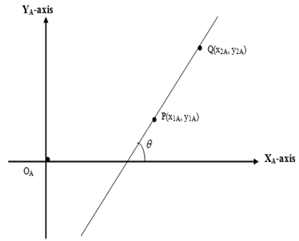
5.2. Slope of an Object LineAn object line is the unique line passing through two points on the Region Coordinate Plane of the region A. We now compute the slope of an object line for this region coordinate plane.
Slope of an object line passing through the two object points P(x1A,y1A) and Q(x2A,y2A) is the real number ma
ma = tan θ = λ.  ,
,
where λ is either +1 or -1 as per the usual sign rule followed in classical geometry.
Therefore, ma = λ. 
= λ. 
= λ.
= λ.
= λ.
= λ. ,
,
(here  means
means which is equal to
  ) = λ.

Thus the slope is neither dependent upon the concerned region nor upon the metric of the region.
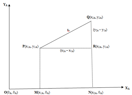
5.3. Distance between Two Object Points (on a Region Coordinate Plane)Distance between two object points on a region coordinate plane can be defined in various ways like in classical geometry. However, we follow the style of Euclidian distance in Region Geometry here.
It can be computed that this distance is an absolute distance in the sense that neither it is dependent upon the concerned region nor upon the metric of the region.
We see that,
d2 = 
= 
= 
= 
= 
= 
This implies that d is neither dependent upon the concerned region nor upon the metric of the region.

The Pythagoras Theorem is thus valid, irrespective of the concerned region or of the metric of the region.
Proposition 5.2
Pythagoras Theorem is valid in every Region Geometry, whatever be the corresponding complete region
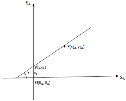
5.4. Object LineConsider the XAYA region coordinate plane corresponding to the complete region A (see Figure 5.1). The general equation of an object line whose slope is ma is yA = ma xA
xA cA .
cA .
Equation of an object line having slope ma and passing through the object point Q(x1A,y1A) is
(yA~y1A) = ma (xA~x1A).
Equation of an object line passing through the two object points P(x1A,y1A) and Q(x2A,y2A) is
(yA ~ y1A) = ma (xA ~ x1A),
where ma =  .
.

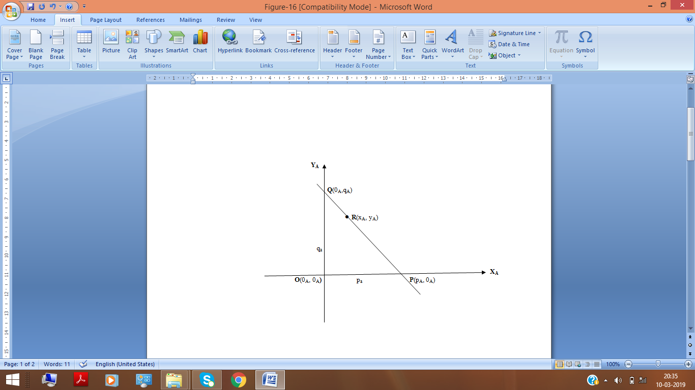
If an object line MN has the intercepts of lengths pa and qa on the X-axes and Y-axes respectively at the points (pA, 0A) and (0A, qA), then the equation of this object line MN will be : 

In the above equations, the variables take values which are objects of the region A. The classical geometry taught at school level is a particular instance of Region Geometry
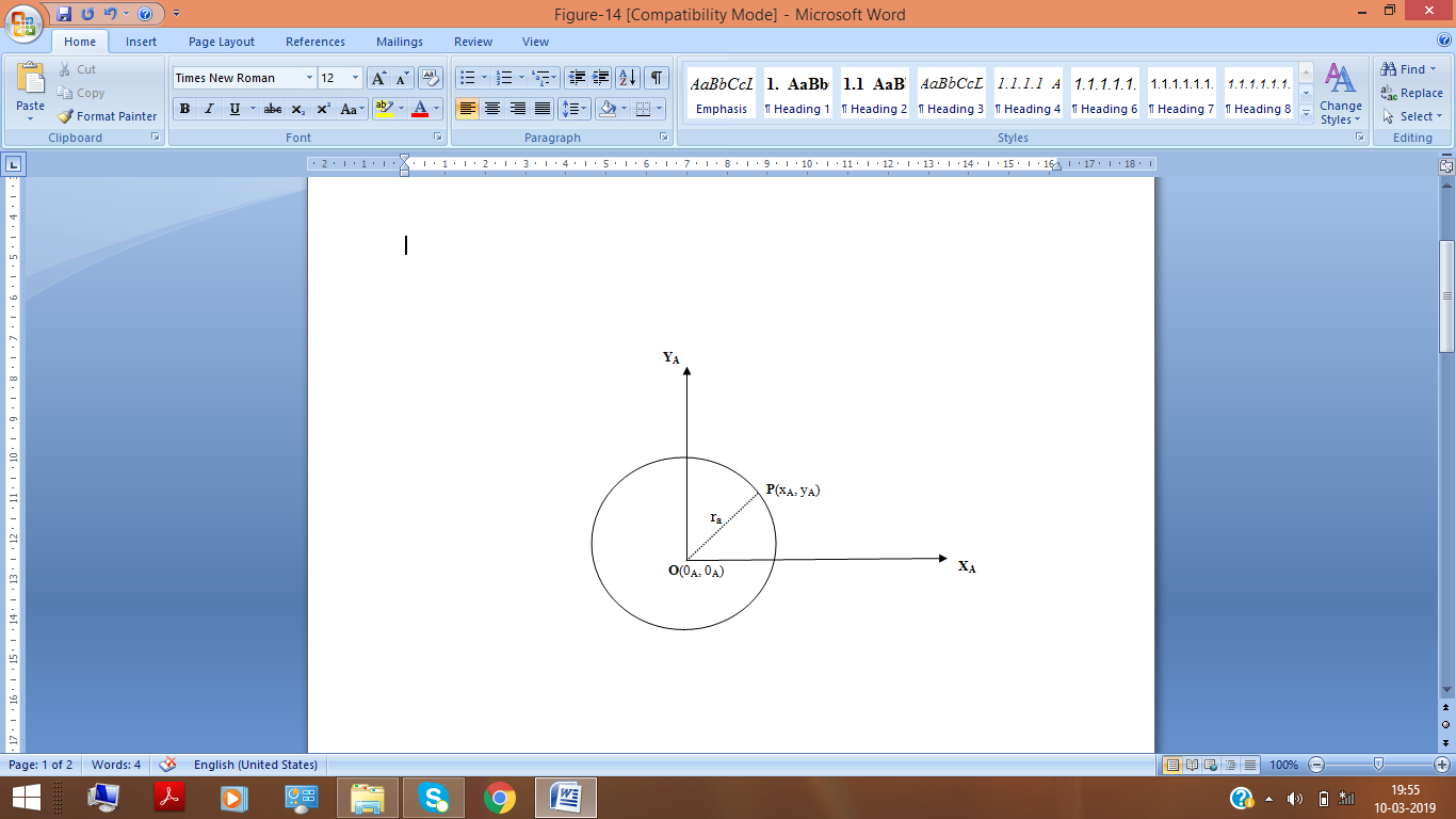
5.5. Object CircleConsider the XAYA region coordinate plane corresponding to the complete region A. Then the equation of an Object Circle (see Figure 5.6) with centre at (0A, 0A) and radius ra (>0) is given by
 ,
,
which can be written as
 .
.

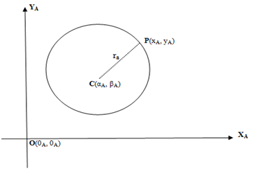
And the equation of the Object Circle (see Figure 5.7) with centre at (αA, βA) and radius ra (>0) is given by
 ,
,
which can be written as


Further study on Region Geometry will be done analogous to the literature of classical geometry 35, in our future works.
For introducing the “Region Calculus”, the very first need of us to recollect an important fact that : Metric Space 36 was discovered after about 250 years of the discovery of Newton Calculus 37, 38, 39, 40, 41. On studying the above five sections of this work, it is very clear now that to develop a new calculus, surely we need an algebraic platform which must be ‘Region’ (not a Division Algebra or any other algebraic structure mentioned in the Key List). Although Newton, known as Father of Calculus, initiated the discovery of Calculus on the algebraic platform R as a Division Algebra, but Fortunately the ‘hidden truth’ is that R is also a Region (failure to which qualification by R could have made the discovery of Calculus delayed!!). The very next point to be noted that while Newton developed calculus, the distance (may be infinitesimal small distance) between the two points x and (x+Δx) on the real line was considered to be equal to the amount {(x+Δx)-x} with no other available options, because the concept of Metric (distance) came into Pure Mathematics after about 250 years of the discovery of Newton Calculus. The concept of the distance amount {(x+Δx)-x} is generalized here with the new concept of ρ((x Δx) ~ x) where ρ is a metric, and the real line of Newton Calculus is replaced in Region Calculus by its generalized concept called by “Object Linear Continuum Line” which is introduced earlier in Section-3.5.
But a natural question at this point arises: Can we develop a calculus over any given region S? We say that if a calculus can be developed over a region S, then this region is to be designated to form a Region Space (see Section 3.2). Thus the same question can be posed in a different way: Can every region form a Region Space? The answer will be clear soon after discussions made in the subsequent subsections.
Consider a partitioned region A = (A, ,*,
,*, ) with respect to the total order relation ‘
 ’. Then the region A forms a Region Space if the following conditions are satisfied:
(i) A is an extended region
(i.e. A is a region and two infinities are also included
to it as permanent guests).
(ii) A is a normed complete metric space with respect to
a norm ║.║ and the corresponding induced metric
ρ(x, y) = ║x~y║, (i.e. ║x║ = ρ(x, 0A) ).
(iii) The norm ║.║ is a 2-to-1 bijective mapping from
A – {0A} to R+.
The subsequent subsections will show that a region calculus can be well developed in a region space. By the phrase “calculus can be developed” means that the basic concepts of Limit, Continuity, Derivatives etc can be developed (in Newton’s Calculus style).
6.1. ‘Region Space’ for Newton Calculus?Consider the partitioned region RR with respect to the crisp order relation “Less Than or Equal To” denoted by the notation “≤”. Choose a norm defined by ║x║ = |x| in RR, and the metric ρ(x, y) =║x-y║= |x-y| in RR. Clearly RR can form a region calculus. It can be observed that this region calculus is nothing but the classical Newton calculus (developed independently by Newton and Leibniz).
The set R of real numbers is so interesting that it very comfortably forms the region RR; and the region RR is so beautiful that it satisfies all the necessary conditions to form a Region Space (an eligible platform on which a calculus can be developed). A division algebra by its definition and independently owned properties does not have so much capability. Consequently, it is clear now that the classical calculus developed independently by Newton and Leibniz happens to be on the particular Region Space RR with respect to a particular order relation “Less Than or Equal To” denoted popularly by the traditional notation “≤” and with respect to the norm defined by ║x║ = |x| in RR, where
the metric ρ(x, y) =║x-y║= |x-y| in RR.
The following facts may be recalled that the metric ρ associated with the norm ║.║ i.e. the metric ρ(x, y) = ║x~y║ has the following special properties:
Although these two beautiful properties were established much later than the discovery of the Newton calculus, but today these can be observed to be true in the ‘Region Space’ of Newton calculus.
We know that a real region which forms a region space is called a “complete region”. We will introduce later that by a complete region, we will always mean one-dimensional complete region (1-D complete region). For instance, the region RR is a complete region with respect to the crisp order relation “Less Than or Equal To” denoted by the notation “≤” and the metric ρ(x, y) = ║ x - y║ = |x-y|, where the norm is the classical norm defined over R. The collection of all the complete regions is called the complete region universe Ʃ.
Before going to introduce the concept of limit and continuity, we recollect quickly few important concepts.
Positive Object and Negative Object
Consider a partitioned complete region A=(A, ,*,
,*, ). In earlier section, three partitions of a region is made which are denoted by A+, A- and {0A} where A is a chain region with respect to a total order relation ‘
 ’. The elements of A+ are said to be positive objects and the elements of A- are said to be negative objects. The object 0A is neither in A+ nor in A-, and so we say that 0A is neither a positive object nor a negative object. The attribute of being positive or negative is called the sign of the object, and the object 0A is not considered to have a sign of its own.
Object Linear Continuum Line

Thus, any point on the Object Linear Continuum Line of the complete region A is called an object point of A.
For developing an Object Line corresponding to a region A, it must be necessary that A forms a region space. Consider the object linear continuum line and the corresponding XA-axis. Since the region A is complete, there are no "points missing" from it (inside or at the boundary). Since A is a chain, every object of A has a unique address on this object linear continuum line and conversely i.e. corresponding to every address (point) on this ‘object linear continuum line’ there is a unique object of the region A. This property is called “Completeness Property” of this complete region A.
Consider a point x on the X-axis of the object linear continuum line corresponding to the region space A. Then for an infinitesimal small positive object ∆x of the region A, the point (x ∆x) will be at a distance ║∆x║ from the point x along the positive direction of X-axis and the point (x ~ ∆x) will be at a distance ║∆x║ from the point x along the negative direction of X-axis. By distance between two objects x and y lying upon the XX1 Object Linear Continuum Line of the complete region A, we mean the corresponding metric distance ρ(x,y) of the normed complete metric space A. By the distance between two objects x and y of the complete region A, we mean the corresponding metric distance ρ(x, y) of the normed complete metric space A. The distance of a positive object xA from the origin is
  = ρ(xA, 0A) = xa, and the distance of a negative object -xA from the origin is = -xa (imposing minus sign). For example, see a collection of consecutive equi-spaced points on the object line as shown in the Figure 6.2 below.

The following theorems follow directly from the above constructions:-
Theorem 6.1
(i) For every positive object x of the region space A, x = ║ x ║ 1A
1A
(ii) For every negative object x of the region space A, x = ~║ x ║ 1A
1A
Theorem 6.2
The unit element 1A of the region space A is at the distance 1 (real integer) on the right side of the zero element 0A on the object linear continuum line of A.
Theorem 6.3
The positive object x of the region space A is located at a distance ║ x ║ from the zero element 0A on the right side of 0A on the object linear continuum line, and the negative object x is located at a distance ║ x ║ from the zero element 0A on the left side of 0A,
Example 6.1
If we choose the region A to be the RR region which is a partitioned region with respect to the crisp order relation “Less Than or Equal To” denoted by the notation “≤”, and if we choose ║x║ = |x| in RR, where
ρ(x, y) =║x-y║= |x-y|,
then it can be observed that the X-axis of the region calculus is the classical X-axis popularly used by us in the Cartesian coordinate system in Newton Calculus, the corresponding linear object continuum is the classical real continuum and the Newton Calculus as a topic becomes an example of region calculus. A region calculus is a generalized model of all the calculus.
6.2. Concept of “Limit” in Region CalculusConsider a Region Space A on which we now develop a region calculus in the Region Space. For this purpose, the basic concepts of any new calculus (of a new differential calculus) are: limit, continuity, differentiability of a function of objects, etc. which we need to introduce first of all in the Region Space (analogous to the classical style of Newton calculus).
 a”
a”We are well aware of the concept of “x  a” in Newton Calculus. In this section we define the notion of “x
  a” in region calculus A, where x, a are in A.
Let us have no confusion about the identity:
a r
r 1A = a
 (r
(r 1A), where r is a real number. Consider an object variable x over the Region Space A = (A,
 ,*,
,*, ). Let a
  A be a fixed object. Suppose that while approaching the object a from its right side along the Object Linear Continuum Line, the object variable x assumes successive object values, out of which some of them for example are :
(a 0.1
0.1 1A), (a
 0.01
0.01 1A), (a
 0.001
0.001 1A), (a
 0.0001
 1A), ….… in its course of journey on the object line X1OX to get close and close to the object a.
Obviously, as the variable x passes through these object points, the value ρ(x, a) becomes less and less and becomes so small that for any positive real number  , no matter however small, ρ(x, a) <
  is satisfied. Let us express this situation using the notation “x
  a+” which means that the object variable x approaches the fixed object a from the right hand side of a (as shown in Figure 6.3). The meaning of ‘right hand side of a’ is clear by definition presented earlier.

Suppose that while approaching the object a from its left side along the Object Linear Continuum Line, the object variable x assumes successive object values, out of which some of them for example are :
(a ~ 0.1 1A), (a ~ 0.01
 1A), (a ~ 0.001
 1A), (a ~ 0.0001
 1A), ……
in its course of journey on the object line X1OX to get close and close to the object a.
Obviously, as x passes through these successive values, the value ρ(x, a) becomes less and less and becomes so small that for any positive real number  , no matter however small, ρ(x, a) <
 is satisfied. Let us express this situation using the notation “x
 a-” which means that the object variable x approaches the fixed object a from the left hand side of a (as shown in Figure 6.4).

By the expression “x tends to a” symbolically written as “x  a”, we mean that given any real
  >0 no matter however small, the successive values of x ultimately satisfy the inequality 0 < ρ(x, a) <
 . It is to be noted that if “x
  a” then ρ(x, a) ≠ 0, i.e. x ≠ a.
Consider an object point a on the Object Linear Continuum Line of the Region Space A = (A, ,*,
,*, ). Analogous to the concept as in Newton Calculus, we define the notion of Neighborhood of an Object Point on the object line.
Let X and Y be two non-null subsets of the Region Space A = (A, ,*,
,*, ) and let f be a function f: X
  Y. Thus f is actually an object valued function of object variable. Then f(x) is said to have a limit l in Y if for any pre-assigned real number
  >0, no matter however small,
  a real number δ > 0 such that
ρ( f(x), l) <  whenever 0 < ρ(x, a) < δ.
We write symbolically as:
 = l, i.e. f(x)
 l as x
 a.
a.
To understand the concept, let us solve the problems posed below.
Problem 6.1
Show that  = l0
= l0 1A in the Region Space given by A = (A,
 ,*,
,*, ).
).
Given real  >0, no matter however small, we need to find out real δ > 0 such that
ρ( 5 x, l0
x, l0 1A) <
1A) <  whenever 0 < ρ(x, 2
 1A) < δ.
i.e. ║5 x ~ l0
 1A║<
1A║<  whenever 0 < ║x ~ 2
 1A║ < δ.
i.e. 5.║x ~ 2 1A║ <
1A║ <  whenever 0 < ║x ~ 2
 1A║ < δ, using properties of A.
Now if we choose δ =  /5, our definition is satisfied.
Hence  = l0
= l0 1A in the Region Space A. Problem 6.2
Show that  = 6
= 6 1A in the Region Space A = (A,
 ,*,
,*, ).
).
Given  >0, no matter however small, we need to find out δ > 0 such that
 <
<  whenever
0 < ρ(x, 3 1A) < δ.
i.e.  <
< 
whenever 0 < ║x ~ 3 1A║ < δ.
Since x 3
3 1A therefore x ≠ 3
 1A and hence
(x ~ 3 1A) ≠ 0A.
Therefore, Cancellation Laws of region algebra can be applied to get the following result :
║ (x  3
3 1A) ~ 6
 1A ║ <
whenever 0 < ║x ~ 3 1A║ < δ.
i.e. ║ x ~ 3 1A║ <
1A║ < 
whenever 0 < ║x ~ 3 1A║ < δ.
Now if we choose δ =  , our definition is satisfied. Hence the result.
The Region Space discussed so far is basically one dimensional Region Space (1-D Region Space) and the corresponding region calculus is also one dimensional. It is because of the reason that in a Region Space any variable x can vary/move along a straight line only. By a ‘complete region’ we shall mean that it is corresponding to a possible development of an 1-D Region Space.
In this section we introduce the concept of ‘Multi-dimensional Region Space’ as a generalization of the concept of ‘Region Space’. In a two-dimensional Region Space (2-D Region Space), a variable z can move along a curve on a plane. The corresponding region calculus is called a 2-D region calculus. In a three-dimensional Region Space (3-D Region Space), a variable w can move along a curve on a 3-D space. The corresponding region calculus is called a 3-D region calculus. Similarly, in an n-D Region Space, a variable µ can move along a curve on a n-D hyperspace. The corresponding region calculus is called an n-D region calculus. Instead of the concept of the extended region, there could be more number of infinities leading to ‘multi-extended region’. The notion of multi-extended region needs to be studied in depth in future. However, let us call a partitioned region to be a multi-extended region if it has more than two infinities. We first of all define n-to-1 Bijective Mapping and Multi-dimensional Region Space.
Consider two non-null sets X and Y. A function
f : X  Y is said to be a ‘n-to-1 Bijective Mapping’ if
(i) f is onto, and
(ii)  y
y  Y,
Y,  a unique subset Sy of X of cardinality n (> 2) such that
  x
x  Sy we have f(x) = y.
Here n could be finite positive integer (> 2) or infinity.
For example, the function f : C-{0} R+ given by
f(z) = |z|2 is a n-to-1 Bijective Mapping, where C is the set of complex numbers.
Consider a partitioned region A = (A, ,*,
,*, ). Then A forms a Multi-dimensional Region Space if the following conditions are satisfied :
(i) A is a multi-extended region.
(ii) A is a normed complete metric space with respect to
a norm ║.║ and the corresponding induced metric
ρ(x, y) = ║x~y║, (║x║ = ρ(x, 0A) ).
(iii) The norm ║.║ is a n-to-1 bijective mapping from
A–{0A} to R+ for some fixed integer n > 2.
6.4. n-D Complete RegionA real region which can form a n-D Region Space is called a “n-D complete region”. A calculus developed out of n-dimensional Region Space is called by n-dimensional region calculus. It may happen that a region can not form an n1-dimensional Region Space, but can well form an n2-dimensional Region Space for some positive integers n1 and n2. In other words, a region may not form an n1-dimensional region calculus, but may well form an n2-dimensional region calculus.
It is to be carefully noted that, a Division Algebra is not a region in general. Consequently a Division Algebra can not become a Region Space in general even if it satisfies all the conditions of Region Space. Given any region G = (G, ,*,
,*, ) over the field (R, +, .), one can immediately attempt to explore whether G forms a Region Space with respect to a defined norm ║.║ and one defined total order relation ‘
 ’. If G forms a Region Space, then a new calculus can be developed in G. The set C of complex numbers does not satisfy the required conditions to become a Region Space with respect to its popular norm
  . Consequently, no 1-D region calculus can be developed in the region C with respect to this norm. It is to be carefully noted that the existing rich ‘Calculus of Complex Variables’ is not an 1-D region calculus.
However, in our future research work we need to explore whether C forms a multi-dimensional Region Space (say, 2-D Region Space) with respect to its popular norm  so that a 2-D region calculus can be developed in C. And if so, then will this 2-D region calculus be the same calculus as the existing rich ‘Calculus of Complex Variables’ of mathematics?
The set of triangular fuzzy numbers (trapezoidal fuzzy numbers) does not form a region with respect to its existing known operators, and consequently it can not offer any region calculus of any dimension to the fuzzy mathematicians. This is one of the major demerits of the notion of triangular fuzzy numbers and trapezoidal fuzzy numbers, some of the drawbacks have been justified in details in 1, 2, 42.
6.5. How Many Distinct 1-D Complete Regions?An interesting question arises :
How many distinct 1-D complete regions exist mathematically in Region mathematics?
To answer this question, first of all we see that given a region A = (A, ,*,
,*, ) over the field (F, +, .) there may (may not) exist more number of regions corresponding to the same set A over the same set F but with different operators
  , *,
, *,  and +, ., respectively.
Even if P = (A, ,*,
,*, ) be a given fixed complete region with respect to the total order relation ‘
 ’ and the norm ║.║, there could be another distinct complete region Q = (A,
 ,*,
,*, ) with respect to a different total order relation or with respect to a different norm or with respect to different pair of total order relation and norm both. There could be many more such complete region (A,
 ,*,
,*, ) in similar ways. However, we will explore this in depth in our future research work.
Thus a given region A = (A, ,*,
,*, ) over the field (F, +, .) may produce more than one distinct complete regions (even retaining the set A, retaining the set F and retaining the operators
  , *,
, *,  and +, ., unchanged), but with different total order relations and different norms, subject to fulfillment of the definition of one dimensional region calculus.
For example, consider the Newton Calculus which is based upon the complete region RR but with respect to the crisp order relation “Less Than or Equal To” denoted by the notation “≤” and the classical norm ║.║ defined by ║x║ = |x| in RR, where the corresponding metric is given by ρ(x, y) =║x-y║= |x-y|. Now, for any real number k>0 we can define a new norm  over the region RR as:
  = k |x|.
It can be observed that the region RR in this case forms a new one dimensional Region Space with respect to this new norm  and the corresponding metric
  which is given by
 = =║x-y║new = k |x - y| , even retaining the same crisp order relation “Less Than or Equal To” (≤).
Thus we can define infinite number of distinct norms mathematically and infinite number of distinct corresponding metrics. Even retaining the same total order relation we can define infinite number of distinct 1-D region calculus mathematically. Newton Calculus is an example of 1-D region calculus which is based upon the platform of the real region space RR.
The existing huge volume of algebraic structures in the subject “ALGEBRA” has few serious hidden gaps and needs fixing in order to validate many of the elementary and important frequently practiced algebraic computations. It is justified in length and established by several examples in 1 that the existing huge volume of algebraic structures in the subject “ALGEBRA” is incomplete to validate many elementary frequently practiced algebraic computations like : square or cube (or nth power) of an algebraic expression, frequently practiced few identities, Cross-Multiplication rule, and many more. None of the algebraic structures of the Key List (as defined above) can validate these computations by their respective definitions and by virtue of their respective properties, except the newly introduced algebraic structure ‘region’. Even an important, very useful and most frequently used Cross-Multiplication rule, which has been being used fluently by the mathematicians and by the scientists of all the STEM subjects for last several centuries, can not be validated (can not be verified) by any individual algebraic structure of the Key List.
Many mathematicians of this century may summarily reject this above statement, because of the strong reason that: “How come the above fact about :Cross-Multiplication Rule” can be true which have been fluently and successfully used by all scientists for several past centuries without having any erroneous or wrong result?’.
This serious gap in the subject Algebra has been discovered and fixed in the work 1. The ‘minimal’ and ‘most useful’ algebraic structure in the subject Algebra is ‘Region’ to validate the frequently practiced algebraic computations, but not any of the existing algebraic structures like : Semi Group, Group, Ring, Integral Domain, Module, Field, Linear Space, Algebra over a field and Extensions, Associative algebra over a field, F-algebra, Division Algebras, Euclidian Hurwitz Algebra, Cayley–Dickson algebra (Octonion Algebra), Clifford Algebra, Quaternion Algebra, universal algebra, etc. Although this statement seems to be unimaginable, unbelievable and impossible, but this genuine fact is established in full length by all possible justifications.
By the birth of the new algebraic structure ‘Region’ which is proved mathematically to be the ‘minimal’ and ‘most important’ algebraic structure, the serious gaps in the giant subject ALGEBRA are fixed by introducing the algebraic structure region. In this work, a new theory called by “Theory of A-numbers” is developed in the Theory of Objects. As mentioned in our earlier work 2 that the classical ‘Theory of Numbers’ is a special case of the “Theory of Objects”. And then an application of the notion of A-numbers is used to introduce the new concept of ‘Region Geometry’. The new notion of im-numbers and compound numbers introduced in Number Theory in our earlier work 2 will play huge role in Pure Mathematics. The notion of im-number is a generalized concept of “imaginary number”, and the notion of compound numbers is a generalized concept of the “complex numbers”.
The concept of ontegers in the Theory of A-numbers is expected to be important in Data Science in this era of AI in particular while dealing with unstructured or semi-structured data. This is our future research work, the present work being purely a theoretical work in Pure Mathematics. The classical concept of ‘Integers’ in the Theory of Numbers are examples of ontegers corresponding to the region RR in the theory of RR-numbers. It may be noted that to represent the omtegers 0A, 1A, 2A, 3A, 4A, 5A, ….., we use the integers 0, 1, 2, 3, 4, ….. and so on. Consequently, instead of saying “integers are special case of ontegers”, it is more appropriate to say “ontegers are extended concept of integers”. In today’s modern Statistics and Data Science, most of the complex data being analysed by the researchers are unstructured or semi-structured data, not the data of R or Rn. Consequently, the collected data are not always from R or Rn, but various types of objects. Todays AI-analysts need more support from Pure Mathematics to deal with unstructured or semi-structured data in their everyday analysis and research activities. The “Region Geometry” is initiated in Pure Mathematics. “Region Geometry” corresponding to the particular region R generates the classical subject “Geometry”. Today the newly born subject :Region Geometry” is in its baby stage, but it is expected that in due time the “Region Geometry” will get fast growth to play good roles in Pure Mathematics, for advanced role in STEM subjects.
At the end section, a new mathematics is introduced entitled ‘Region Calculus’ on defining a notion of ‘Region Space’. The classical calculus developed independently by Newton and Leibniz is based on the set R of real numbers, extended with two infinities, and then took its shape further with functions of complex variables, vector calculus, tensor calculus, etc. The growth of classical calculus at every stage required fluent applications of various properties of the set R of real numbers. Using the properties of a ‘field’ or a ‘division algebra’ or any existing standard algebra, the classical calculus can not have the validity of its all fluent results as justified in length. To fix these important gaps, a new algebraic structure region is introduced. Fortunately the set R happens to be a trivial example of real region and the mathematicians enriched the classical calculus using the properties of region R, although ‘unknowingly’. The major contribution in this work is that we have precisely identified: ‘What are the minimum properties which need to be satisfied by a set A so that a calculus can be developed over A?’. Consequently we have introduced the notion of ‘Region Space’ as a general minimal platform on which a calculus can be developed. It has been explained that the platform R of classical calculus is actually a Region Space, and consequently there was no hurdles to discover calculus in 1665-1666. For a non-example, the set of all triangular fuzzy numbers do not form a real region with respect to its commonly used operators, and hence can not open any platform to develop any fuzzy differential calculus and fuzzy integral calculus over it in the style of the classical calculus. The requirements are precisely identified as a checklist before making any attempt to develop any new calculus over a given set. We presume that our future computations (be it in this solar system or in other, be it in this universe or in other of the multiverse) may not be sufficiently covered by or compatible with our classical calculus. Consequently, the very first job is to define the general structure of a mathematical space which is a minimum requirement for making an attempt to develop any new calculus over it. It is justified that mathematically there exist an infinite number of distinct complete regions and there exist infinite number of distinct 1-D region calculus. Then we generalize the concept of Region Space by defining ‘multi-dimensional Region Space’. The simple term Region Space is basically one dimensional Region Space (1-D Region Space) and the corresponding region calculus is also one dimensional region calculus. In a Region Space any variable x can vary/move along a straight line only, i.e. if x a in a complete region, it means that x is being driven along a straight line. The concept of ‘Multi-dimensional Region Space’ is a generalization of the concept of ‘Region Space’. In a two-dimensional Region Space (2-D Region Space), a variable z can move along a curve on a plane. The corresponding region calculus is called a 2-D region calculus. In a three-dimensional Region Space (3-D Region Space), a variable w can move along a curve on a 3-D space. The corresponding region calculus is called a 3-D region calculus. Similarly, in an n-D Region Space, a variable µ can move along a curve on a n-D hyperspace. The corresponding region calculus is called an n-D region calculus (i.e. n-dimensional region calculus). It may happen that a region can not form an n1-dimensional Region Space, but can well form an n2-dimensional Region Space. In other words, a region may not form an n1-dimensional region calculus, but may form an n2-dimensional region calculus. It is to be carefully noted that mathematically an arbitrary Division Algebra is not a region in general by virtue of its definition and properties. Consequently an arbitrary Division Algebra can not qualify to become a Region Space in general. The proposed theory of Region Calculus helps us to study for any arbitrary region G = (G,
 ,*,
,*, ) over the field (R, +, .) to explore whether G forms a Region Space with respect to a suitable norm ║.║ and a suitable total order relation ‘
 ’. If G forms a Region Space, then a new calculus can be well developed in G. However, the set C of complex numbers does not satisfy the required conditions to become a Region Space with respect to its popular norm
  . Consequently, no 1-D region calculus can be developed in the region C. However, in our future research work we need to explore whether C forms a multi-dimensional Region Space (2-D Region Space) with respect to its popular norm
  so that a 2-D region calculus can be developed in C. The set of triangular fuzzy numbers (trapezoidal fuzzy numbers) does not form a region with respect to its existing known operations, and consequently it can not offer any region calculus of any dimension to us. This is one of the major demerits of the notion of triangular fuzzy numbers and trapezoidal fuzzy numbers, the drawbacks being justified in details in our earlier work. A Region Space is a base-platform on which one can develop a new calculus. In other words, a calculus can not be developed without a Region Space, called a base-platform of the calculus. It is observed that the existing rich calculus of Newton is a particular case of Region Calculus (i.e. one instance of Region Calculus). Consequently, we can view Region Calculus as a generalized model of all calculusus. Newton calculus is now observed to be a calculus based on region R, not on the division algebra R because the Division Algebra R can not support the algebraic computations involved in Newton Calculus by virtue of the definition and properties of ‘Division Algebra’. However, the following two problems are open future problems of us:-(i) Today it is observed that in Newton Calculus, the metric space was the metric ρ defined by ρ(x, y) =║x-y║= |x-y|, over the region R. How to obtain another new calculus using another metric space over the region R. (ii) to discover an example of a new calculus over any other region A (other than the region R). The complete work reported here launches a new topic “Region Mathematics” in the giant subject Pure Mathematics, and it will certainly open new gates for broader applications of Pure Mathematics, will cater to the future research activities in all the STEM subjects, including Data Science, AI and modern Statistics. This work is just the beginning of “Region Mathematics”.
The author is thankful to both the Referees for their valuable suggestions for improvement of the first version of the manuscript.
| [1] | Biswas, Ranjit., The existing huge volume of algebraic structures in the subject “ALGEBRA” has few serious hidden gaps and needs fixing in order to validate many of the elementary and important frequently practiced algebraic computations, Indonesian Journal of Mathematics and Analysis, 2026, Vol.1, 35–69 (Open Access). | ||
| In article | View Article | ||
| [2] | Biswas, Ranjit., ‘Object Theory’: The Classical ‘Number Theory’ is a Special Case, Turkish Journal of Analysis and Number Theory, 2026, Vol. 14, No. 1, pp 6-22 (Open Access) (Available online at http://pubs.sciepub.com/tjant/14/1/2). | ||
| In article | View Article | ||
| [3] | Fraenkel, A., Bar-Hillel, Y., and Lev., Foundations of Set Theory. North Holland, Amsterdam, 1973. | ||
| In article | |||
| [4] | Apostol, Tom M., Introduction to Analytic Number Theory. Springer-Verlag. Heidelberg Berlin, 1976. | ||
| In article | View Article | ||
| [5] | Bourbaki, Nicolas., Elements of the History of Mathematics. Springer-Verlag, Berlin, 1994. | ||
| In article | |||
| [6] | Bourbaki, Nicolas., Elements of Mathematics: Algebra I. New York: Springer-Verlag, 1998. | ||
| In article | |||
| [7] | Dixon, G.M., Division Algebras: Octonions Quaternions Complex Numbers and the Algebraic Design of Physics. Kluwer Academic Publishers, Dordrecht, 2010. | ||
| In article | |||
| [8] | Herstein, I. N., Topics in Algebra. Wiley Eastern Limited. New Delhi, 2001. | ||
| In article | |||
| [9] | Hungerford, T., Algebra, Graduate Texts in Mathematics, Vol. 73, Springer-Verlag, New York, 1974. | ||
| In article | View Article | ||
| [10] | Jacobson, N., Basic Algebra I. 2nd Ed., W. H. Freeman & Company Publishers, San Francisco, 1985. | ||
| In article | |||
| [11] | Jacobson, N., Basic Algebra II. 2nd Ed., W. H. Freeman & Company Publishers, San Francisco, 1989. | ||
| In article | |||
| [12] | Jacobson, N., The Theory of Rings. American Mathematical Society Mathematical Surveys. Vol.I. American Mathematical Society. New York, 1943. | ||
| In article | View Article | ||
| [13] | Lang, Serge., Undergraduate Algebra. (3rd ed.). Berlin, New York: Springer-Verlag, 2005. | ||
| In article | |||
| [14] | Leonard E. Dickson, History of the Theory of Numbers (Vol-1), Washington Carnegie Institution of Washington, 1919. | ||
| In article | |||
| [15] | Leonard E. Dickson, History of the Theory of Numbers (Vol-2), Washington Carnegie Institution of Washington, 1920. | ||
| In article | |||
| [16] | Leonard E. Dickson, History of the Theory of Numbers (Vol-3), Washington Carnegie Institution of Washington, 1923. | ||
| In article | |||
| [17] | Nahin, Paul J., An Imaginary Tale: The Story of √−1, Princeton University Press, ISBN 978-0691127989, retrieved 20 April 2011. | ||
| In article | |||
| [18] | Ore, Øystein., Number theory and its history, New York, McGraw-Hill Book Co. 1948. | ||
| In article | |||
| [19] | Reyes, Mitchell., The Rhetoric in Mathematics: Newton, Leibniz, the Calculus, and the Rhetorical Force of the Infinitesimal. Quarterly Journal of Speech. Vol. 90. 159-184, 2004. | ||
| In article | View Article | ||
| [20] | Robbins, Herbert. and Courant, Richard., What is Mathematics?: An Elementary Approach to Ideas and Methods. Second edition, Oxford University Press, New York, 1986. | ||
| In article | |||
| [21] | Rosen, Kenneth H., Elementary Number Theory (6th ed.). Pearson Education. US, 2010. | ||
| In article | |||
| [22] | Rudin, Walter., Real and Complex Analysis. McGraw Hills Education, India, 2006. | ||
| In article | |||
| [23] | Sardar, Ziauddin., Ravetz, Jerry., Loon, Borin Van Loon., Introducing Mathematics. Icon Books Ltd, London, 2015 Reprint edition. | ||
| In article | |||
| [24] | Silverman, Joseph H., A Friendly Introduction to Number Theory, Pearson Education, 2001. | ||
| In article | |||
| [25] | Simmons, G. F., Introduction to Topology and Modern Analysis. McGraw Hill, New York, 1963. | ||
| In article | |||
| [26] | Stillwell, John., Elements of Number Theory, Springer-Verlag New York, 2010. | ||
| In article | |||
| [27] | Van der Waerden and Bartel Leendert., Algebra. Springer-Verlag, New York, 1991. | ||
| In article | View Article | ||
| [28] | Vinogradov, I.M., Elements of Number Theory (reprint of the 1954 ed.). Mineola, NY: Dover Publications. Mineola, New York, 2003. | ||
| In article | |||
| [29] | Waerden, Bartel Leenert Van der., Algebra. Springer-Verlag, New York, 1991. | ||
| In article | |||
| [30] | Watkins, J. J., Number theory: a historical approach, Princeton University Press, 2013. | ||
| In article | |||
| [31] | Biswas, Ranjit., Birth of Compound Numbers, Turkish Journal of Analysis and Number Theory. Vol.2(6). pp 208-219, 2014. | ||
| In article | View Article | ||
| [32] | Davenport, H., The Higher Arithmetic, Cambridge University Press, 2008. | ||
| In article | View Article | ||
| [33] | Edwards, Harold M., Fermat's Last Theorem: a Genetic Introduction to Algebraic Number Theory. Graduate Texts in Mathematics. Springer-Verlag. New York, 2000. | ||
| In article | |||
| [34] | Hardy, G.H., Wright, Edward M., Roger Heath-Brown, Silverman, Joseph. and Wile, Andrew., Introduction to the Theory of Numbers. (6th Edition) Oxford University Press, UK, 2008. | ||
| In article | |||
| [35] | Boyer, Carl B., History of Analytic Geometry. Dover Publications, Inc., Mineola, New York, 2004. | ||
| In article | |||
| [36] | Copson, E.T., Metric Spaces. Cambridge University Press, 1968. | ||
| In article | View Article | ||
| [37] | Acheson, David., The Calculus Story: A Mathematical Adventure, First Edition, Oxford University Press, UK, 2017. | ||
| In article | |||
| [38] | Baron, Margaret E. (2003). The origins of the infinitesimal calculus. Dover Publications, Inc., Mineola, New York. | ||
| In article | |||
| [39] | Boyer, Carl B. and Merzbach, Uta C., A History of Mathematics, 3rd Edition. John Wiley & Sons, Hoboken, New Jersey, 2011. | ||
| In article | |||
| [40] | Boyer, Carl B., The History of the Calculus and Its Conceptual Development. Dover Publications, Inc., Mineola, New York, 1959. | ||
| In article | |||
| [41] | Cajori, Florian., A History of Elementary Mathematics – With Hints on Methods of Teaching. Read Books. UK, 2010. | ||
| In article | |||
| [42] | Biswas, Ranjit., Is ‘Fuzzy Theory’ An Appropriate Tool For Large Size Problems ?. in the book-series of SpringerBriefs in Computational Intelligence. Springer. Heidelberg, 2016. | ||
| In article | View Article | ||
Published with license by Science and Education Publishing, Copyright © 2026 Ranjit Biswas
 This work is licensed under a Creative Commons Attribution 4.0 International License. To view a copy of this license, visit
http://creativecommons.org/licenses/by/4.0/
This work is licensed under a Creative Commons Attribution 4.0 International License. To view a copy of this license, visit
http://creativecommons.org/licenses/by/4.0/
| [1] | Biswas, Ranjit., The existing huge volume of algebraic structures in the subject “ALGEBRA” has few serious hidden gaps and needs fixing in order to validate many of the elementary and important frequently practiced algebraic computations, Indonesian Journal of Mathematics and Analysis, 2026, Vol.1, 35–69 (Open Access). | ||
| In article | View Article | ||
| [2] | Biswas, Ranjit., ‘Object Theory’: The Classical ‘Number Theory’ is a Special Case, Turkish Journal of Analysis and Number Theory, 2026, Vol. 14, No. 1, pp 6-22 (Open Access) (Available online at http://pubs.sciepub.com/tjant/14/1/2). | ||
| In article | View Article | ||
| [3] | Fraenkel, A., Bar-Hillel, Y., and Lev., Foundations of Set Theory. North Holland, Amsterdam, 1973. | ||
| In article | |||
| [4] | Apostol, Tom M., Introduction to Analytic Number Theory. Springer-Verlag. Heidelberg Berlin, 1976. | ||
| In article | View Article | ||
| [5] | Bourbaki, Nicolas., Elements of the History of Mathematics. Springer-Verlag, Berlin, 1994. | ||
| In article | |||
| [6] | Bourbaki, Nicolas., Elements of Mathematics: Algebra I. New York: Springer-Verlag, 1998. | ||
| In article | |||
| [7] | Dixon, G.M., Division Algebras: Octonions Quaternions Complex Numbers and the Algebraic Design of Physics. Kluwer Academic Publishers, Dordrecht, 2010. | ||
| In article | |||
| [8] | Herstein, I. N., Topics in Algebra. Wiley Eastern Limited. New Delhi, 2001. | ||
| In article | |||
| [9] | Hungerford, T., Algebra, Graduate Texts in Mathematics, Vol. 73, Springer-Verlag, New York, 1974. | ||
| In article | View Article | ||
| [10] | Jacobson, N., Basic Algebra I. 2nd Ed., W. H. Freeman & Company Publishers, San Francisco, 1985. | ||
| In article | |||
| [11] | Jacobson, N., Basic Algebra II. 2nd Ed., W. H. Freeman & Company Publishers, San Francisco, 1989. | ||
| In article | |||
| [12] | Jacobson, N., The Theory of Rings. American Mathematical Society Mathematical Surveys. Vol.I. American Mathematical Society. New York, 1943. | ||
| In article | View Article | ||
| [13] | Lang, Serge., Undergraduate Algebra. (3rd ed.). Berlin, New York: Springer-Verlag, 2005. | ||
| In article | |||
| [14] | Leonard E. Dickson, History of the Theory of Numbers (Vol-1), Washington Carnegie Institution of Washington, 1919. | ||
| In article | |||
| [15] | Leonard E. Dickson, History of the Theory of Numbers (Vol-2), Washington Carnegie Institution of Washington, 1920. | ||
| In article | |||
| [16] | Leonard E. Dickson, History of the Theory of Numbers (Vol-3), Washington Carnegie Institution of Washington, 1923. | ||
| In article | |||
| [17] | Nahin, Paul J., An Imaginary Tale: The Story of √−1, Princeton University Press, ISBN 978-0691127989, retrieved 20 April 2011. | ||
| In article | |||
| [18] | Ore, Øystein., Number theory and its history, New York, McGraw-Hill Book Co. 1948. | ||
| In article | |||
| [19] | Reyes, Mitchell., The Rhetoric in Mathematics: Newton, Leibniz, the Calculus, and the Rhetorical Force of the Infinitesimal. Quarterly Journal of Speech. Vol. 90. 159-184, 2004. | ||
| In article | View Article | ||
| [20] | Robbins, Herbert. and Courant, Richard., What is Mathematics?: An Elementary Approach to Ideas and Methods. Second edition, Oxford University Press, New York, 1986. | ||
| In article | |||
| [21] | Rosen, Kenneth H., Elementary Number Theory (6th ed.). Pearson Education. US, 2010. | ||
| In article | |||
| [22] | Rudin, Walter., Real and Complex Analysis. McGraw Hills Education, India, 2006. | ||
| In article | |||
| [23] | Sardar, Ziauddin., Ravetz, Jerry., Loon, Borin Van Loon., Introducing Mathematics. Icon Books Ltd, London, 2015 Reprint edition. | ||
| In article | |||
| [24] | Silverman, Joseph H., A Friendly Introduction to Number Theory, Pearson Education, 2001. | ||
| In article | |||
| [25] | Simmons, G. F., Introduction to Topology and Modern Analysis. McGraw Hill, New York, 1963. | ||
| In article | |||
| [26] | Stillwell, John., Elements of Number Theory, Springer-Verlag New York, 2010. | ||
| In article | |||
| [27] | Van der Waerden and Bartel Leendert., Algebra. Springer-Verlag, New York, 1991. | ||
| In article | View Article | ||
| [28] | Vinogradov, I.M., Elements of Number Theory (reprint of the 1954 ed.). Mineola, NY: Dover Publications. Mineola, New York, 2003. | ||
| In article | |||
| [29] | Waerden, Bartel Leenert Van der., Algebra. Springer-Verlag, New York, 1991. | ||
| In article | |||
| [30] | Watkins, J. J., Number theory: a historical approach, Princeton University Press, 2013. | ||
| In article | |||
| [31] | Biswas, Ranjit., Birth of Compound Numbers, Turkish Journal of Analysis and Number Theory. Vol.2(6). pp 208-219, 2014. | ||
| In article | View Article | ||
| [32] | Davenport, H., The Higher Arithmetic, Cambridge University Press, 2008. | ||
| In article | View Article | ||
| [33] | Edwards, Harold M., Fermat's Last Theorem: a Genetic Introduction to Algebraic Number Theory. Graduate Texts in Mathematics. Springer-Verlag. New York, 2000. | ||
| In article | |||
| [34] | Hardy, G.H., Wright, Edward M., Roger Heath-Brown, Silverman, Joseph. and Wile, Andrew., Introduction to the Theory of Numbers. (6th Edition) Oxford University Press, UK, 2008. | ||
| In article | |||
| [35] | Boyer, Carl B., History of Analytic Geometry. Dover Publications, Inc., Mineola, New York, 2004. | ||
| In article | |||
| [36] | Copson, E.T., Metric Spaces. Cambridge University Press, 1968. | ||
| In article | View Article | ||
| [37] | Acheson, David., The Calculus Story: A Mathematical Adventure, First Edition, Oxford University Press, UK, 2017. | ||
| In article | |||
| [38] | Baron, Margaret E. (2003). The origins of the infinitesimal calculus. Dover Publications, Inc., Mineola, New York. | ||
| In article | |||
| [39] | Boyer, Carl B. and Merzbach, Uta C., A History of Mathematics, 3rd Edition. John Wiley & Sons, Hoboken, New Jersey, 2011. | ||
| In article | |||
| [40] | Boyer, Carl B., The History of the Calculus and Its Conceptual Development. Dover Publications, Inc., Mineola, New York, 1959. | ||
| In article | |||
| [41] | Cajori, Florian., A History of Elementary Mathematics – With Hints on Methods of Teaching. Read Books. UK, 2010. | ||
| In article | |||
| [42] | Biswas, Ranjit., Is ‘Fuzzy Theory’ An Appropriate Tool For Large Size Problems ?. in the book-series of SpringerBriefs in Computational Intelligence. Springer. Heidelberg, 2016. | ||
| In article | View Article | ||