In this paper, the bi-quintic B-spline base functions are modified on a general 2-dimensional problem and then they are applied to two-dimensional Diffusion problem in order to obtain its numerical solutions. The computed results are compared with the results given in the literature.
In this paper, we will consider two dimensional Diffusion equation of the form
 | (1) |
with the initial condition
 | (2) |
and boundary conditions
 | (3) |
 | (4) |
 | (5) |
 | (6) |
on the region  The exact solution of this problem is 1
 | (7) |
where K is a diffusion coefficent.
The finite element method has been widely applied to physics, solid and fluid mechanics, engineering, medicine and so on 2, 3, 4, 5, 6, 7, 8, 9, 10, 11, 12. Particularly, Kasi and Koneru 13 have used the Galerkin finite element method for onedimensional and two-dimensional time dependent problems by modifying bicubic B-spline base functions. Moon et al. 1 have obtained a non-separable solution of the diffusion equation based on the Galerkin’s method using cubic splines. Tavakoli and Davami 14 have developed a parallel unconditionally stable fully explicit finite difference scheme for solution of the diffusion equation. Ang 15 has proposed a boundary integral equation method for the numerical solution of the two-dimensional diffusion equation subject to a non-local condition. Velivelli and Bryden 16 have examined cache optimization for the Lattice Boltzmann method in both serial and parallel implementations by utilizing the two-dimesional diffusion equation. Aboanber and Hamada 17 have developed a generalized Runge-Kutta method for the numerical integration of the stiff space-time diffusion equations. Bhaskar et al. 18 have developed Heatlets, the fundamental solutions of heat equation using wavelets, for numerically solving inhomogeneous and homogeneous initial value problems of diffusion equation on unbounded domains. Sterk and Trobec 19 have given the derivation and implementation of a numerical solution of a time-dependent diffusion equation in detail, based on the meshless local Petrov-Galerkin method.
In this paper, we have first modified bi-quintic b-spline functions on the boundary of a general two dimensional dimensional problem and used them to obtain numerical solutions of the Diffusion problem by the Galerkin finite element method. The modified bi-quintic B-splines are used as basis functions and rectangles as element shapes.
We try a bi-quintic B-spline function of the form
 |
as an approximation solution to two dimensional diffusion problem. In order to find an approximate solution in the above form to the problem by the Galerkin method, first of all we have to redefine the B-spline basis functions into a new set of functions, namely modified bi-quintic B-spline functions. This redefining process was successfully applied to cubic B-spline functions to obtain modified bi-cubic B-spline functions 13. The newly obtained set of modified functions are identically zero on the boundary of the given problem. It should be pointed out that this process is necessary, since B-spline basis functions Bi(x)(i = −2(1)(n + 2) in the x-direction and the B-spline basis functions Bj(y)(j = −2(1)(m + 2) in the y-direction are not zero on the boundary of the problem. After the redefining process of the basis functions, we can now try the modified bi-quintic B-spline functions of the form
 |
as its approximate solution, where  and
and  are the quintic B-splines to be modified only on the boundary in the x and y- directions, respectively. Since all of the modified quintic B-splines are zero on the boundary of the problem, non-homogenous boundary conditions are satisfied by the term
The rectangular region D of the problem is subdivided into a number of uniform rectangular finite elements of sides  and
and  by the knots
  where
where 
 An approximation
  with quintic B-spline functions to
  is taken of the form
 | (8) |
where  are the amplitudes of bi-quintic B-splines
  given by
 | (9) |
and Bi(x) is defined as
 |
20. Bj(y) can easily be found by replacing i with j and x with y. Figure 1 depicts a region, where hx = hy = 1, so that it is divided into finite elements by the integer knots (i, j), and a single bi-quintic B-spline B33 which peaks on the point (3, 3) and also covers a total of 36 square elements. When the entire set of bi-quintic splines Bij, each of which peaks on a knot (i, j), where 0 ≤ i ≤ 6, 0 ≤ j ≤ 6, are added to this figure, a total of 36 splines cover each finite element 21.

To show how to modify bi-quintic spline functions on the boundary, we consider the two-dimensional general linear equation of the form
 | (10) |
subject to the initial condition
 | (11) |
and boundary conditions
 | (12) |
 | (13) |
 | (14) |
 | (15) |
where 
 and
and 


 are given functions, D is a rectangular region in R2 with boundary ∂D.
Now, it is supposed that both the x-space variable domain and y-space variable domain of the system (10)-(15) are divided into n and m subintervals, respectively, by the set of n + 1 distinct grid points  and m + 1 distinct grid points
  such that
 |
Since a quintic B-spline function covers six consecutive elements, we add ten additional grid points 


 in the x-direction and ten additional grid points


 in the y-direction such that
 |
 |
 |
 |
To find an approximate solution in the form of Eq. (8) to the problem given by Eqs. (10)-(15) with the Galerkin method, we do need to redefine the basis functions into a new set of basis functions which all vanish on ∂D. The redefining process of the basis functions is done in the following three steps.
Step 1. The approximate solution  given by Eq. (8) can also be written as 13
 | (16) |
where
 | (17) |
Allowing the approximate solution  given by Eq. (16) to satisfy the boundary conditions (14) and (15) and eliminating
  and
and  from the resulting equations, we obtain
 | (18) |
where
 | (19) |
 | (20) |
 | (21) |
Step 2. By evaluating the expression  given by Eq. (17) at
  and
and  and eliminating
  and
and  from the resulting equations, we obtain
 | (22) |
where
 | (23) |
 | (24) |
 | (25) |
Step 3. Finally, substituting  in Eq. (22) into Eq. (18) and allowing the resulting equation to satisfy the boundary conditions (12) and (13), we obtain
 | (26) |
where
 | (27) |
Applying exactly the same three steps, but now writing the approximate solution (8) as 13
 | (28) |
where
 | (29) |
we obtain
 | (30) |
where
 | (31) |


By taking the average of Eq. (27) and Eq. (31), we obtain the general approximation  to
to  of the form
 | (32) |
where the new set of basis functions are  for
for 
 which all vanish on
  and
and  given in Eq. (32) satisfies the boundary conditions given by Eqs. (12)-(15). The profiles of the modified quintic B-splines are shown in Figure 2 for 4 elements.
In this section, we will try to obtain the numerical solutions of the diffusion problem given by Eqs. (1)-(6) using the Galerkin finite element method with the modified bi-quintic B-spline base functions. The diffusion equation is integrated in space variables x and y. To apply the method to the problem, first of all we need to construct the weak form of the problem.
3.1. Weak Form of the Model ProblemFor this purpose, all terms in Eq. (1) are taken to the right hand side of the equation and then multiplied by the weight function Ψ(x, y). Finally, by integrating the resulting equation over the region D and setting it to zero, we get
 | (33) |
where  for k = 0(1)n and l = 0(1)m. By applying the Green Theorem (see, e.g. Reddy 22) to Eq. (33), the weak form of the model problem in the global coordinate system is obtained as follows
 | (34) |
To change from the global coordinate system into the local one, we use the transformations  and
and  Thus, the weak form (34) transforms to the form
 | (35) |
In this subsection, the numerical solutions of the model problem are obtained by the Galerkin finite element method using the modified bi-quintic Bspline basis functions. The numerical scheme is implemented by dividing the region  into
into  and
and  elements. The obtained solutions are compared with those existing in the literature and tabulated with error norms
  and
and  In all numerical calculations, the coefficient
  in Eq. (1) is taken as
For this, the approximate solution  for each element is written in the weak form (35) and then a coefficient matrix is obtained for each element. By combining the coefficient matrix for each element, we obtain an algebraic equation in the form
 | (36) |
and an iterative equation in the form
 | (37) |
 | (38) |
 | (39) |
 | (40a) |
 | (41) |
where i, j, k, l = 0(1)n, il = j(n + 1) + i and jl = l(n + 1) + k
 | (42) |
where i, j, k, l = 0(1)n, il = j(n + 1) + 1 and jl = l(n + 1) + k
 | (43) |
where i, j = 0(1)1, il = j(n + 1) + 1.
The division of the region into 4×4=16 elements
If the solution domain D of the problem is equally divided into 4×4 = 16 elements, 16 squares having the sides of hx = hy = h = 1/4 are obtained. If the approximate solution  is constructed for each element, a total number of 7 × 7 = 49 global element parameters over the region D are obtained depending on the local element parameters αi(t) and βj(t), (i, j =−1(1)5). It is obvious that we need to find the global element parameters Ai(t), (i = 1(1)49) in order to obtain the approximate solution
  for each element. By solving these algebraic equations, element parameters Ai(t), (i=1(1)49) are obtained at times t = 0.0 and t = 1.0.The obtained element parameters are put in their places in the element equations, and then the approximate solution
  for each element at times t = 0.0 and t = 1.0 is found.
The division of the region into 10×10=100 elements
Now the solution domain D of the problem is equally divided into 10 × 10 = 100 elements, 100 squares having the sides of hx = hy = h = 1/10 are obtained.
As in 4 × 4 = 16 elements, if the approximate solution  is constructed for each element, a total number of 13×13 = 169 global element parameters over the region D are obtained depending on the local element parameters
  and
and  (i = −1(1)11). It is obvious that we need to find the global element parameters
  (i = 1(1)49) in order to obtain the approximate solution
  for each element. For this, the approximate solution
  for each element is written in the weak form (35) and then a coefficient matrix is obtained for each element. By combining the coefficient matrices for each element, first we obtain an algebraic equation in the form Eq. (36) then an iterative equation in the form of Eq. (38) by applying forward difference and Crank-Nicolson finite difference formula to Eq. (37). By solving these equations with the help of a computer program we obtain the global element parameters
  (i = 1(1)169) at times t = 0.0 and t = 1.0, respectively. These obtained element parameters are put in their places in the element equations, and then the approximate solutions
  for each element at times t = 0.0 and t = 1.0 are found.
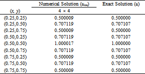
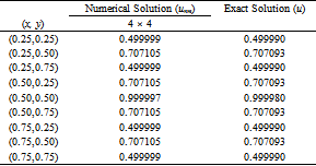
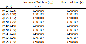
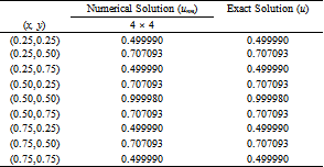
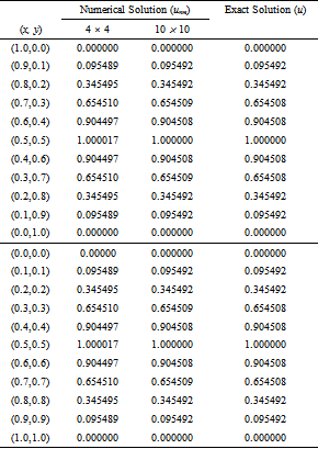
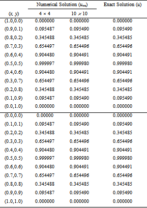
The obtained numerical results by the present method using the modified bi-quintic B-splines have been displayed and also compared with its exact ones in Table 3 – Table 6. It is obviously seen from the tables that the numerical results are in good agreement with the exact ones. Figure 3 and Figure 4 show graphically how closely the approximate solution  matches with the exact solution
  at times t = 0.0 and t = 0.05, respectively. Since the numerical solution is very close to the exact solution, their graphs are indiscriminately similar to each other. In Table 5 and Table 6, the numerical solutions obtained by the Galerkin finite element method with modified biquintic B-spline basis functions are compared with the exact ones at times t = 0.0 and t = 1.0, respectively.


In order to measure how good the numerical solutions obtained by the Galerkin finite element method with the bi-quintic B-spline basis functions, the error norms  and
and  defined as
 |
 |
are computed and tabulated in Table 7. In  and
and 
 is the number of inner points,
  and
and  are the exact and approximate solutions at the point i., respectively. The error norms
  and
and  are computed by taking the values
  and
and  at 41×41 = 1681(=
 ) points obtained by dividing the region D = [0, 1] × [0, 1] into 40 equal elements in the directions x and y. As seen from the table, the approximate solutions become better as the number of elements increase.
In this paper, a modified bi-quintic B-spline finite element method is proposed and successfully applied to two dimensional Diffusion problem to obtain its numerical solutions. The agreement between our numerical results and the exact solution is satisfactorily good. The obtained numerical results showed that the present method is a remarkably successful numerical technique and can also be applied to a large number of physically important two dimensional non-linear problems.
| [1] | B. S. Moon, D. S. Yoo, Y.H. Lee, I.S. Oh, J.W. Lee, D.Y. Lee and K.C. Kwon, A non-separable solution of the diffusion equation based on the Galerkin’s method using cubic splines , Appl. Math. and Comput., 217 (2010) 1831-1837. | ||
| In article | View Article | ||
| [2] | D. L. Logan, A First Course in the Finite Element Method, Thomson Learning, part of the Thomson Corporation, New York, 2007. | ||
| In article | |||
| [3] | M. A. Bhatti, Fundamental Finite Element Analysis and Applications: with Mathematica and Matlab Computations, John Wiley & Sons, Inc., New York, 2005. | ||
| In article | View Article | ||
| [4] | J.N. Reddy, An introduction to Nonlinear Finite Element Analysis, Oxford University Press, New York, 2008. | ||
| In article | |||
| [5] | E. G. Thompson, Introduction To The Finite Element Method, Theory, Programming, and Applications, John Wiley Sons, Inc., USA, 2005. | ||
| In article | |||
| [6] | J. Wu, X. Zhang, Finite Element Method by Using Quartic B-Splines, Numerical Methods for Partial Differential Equations, 10 (2011) 818-828. | ||
| In article | View Article | ||
| [7] | O.C. Zienkiewicz, The finite element method, McGraw-Hill, London, 1977. | ||
| In article | View Article | ||
| [8] | S.Kutluay, A. Esen, I.Dağ, Numerical solutions of the Burgers equation by the least-squares quadratic B-spline finite element method, J Comput Appl Math 167 (2004) 21-33. | ||
| In article | View Article | ||
| [9] | H.Bateman, Some recent researcher on the motion of fluids, Mon. Weather Rev. 43 (1915) 163-170. | ||
| In article | View Article | ||
| [10] | J.M. Burger, A matematical model illustrating the theory of turbulence, Advances in Applied Mechanics I, Academic Press, New York, (1948) 171-19. | ||
| In article | View Article | ||
| [11] | J.D. Cole, On A Quasi Linear Parabolic Equaion Occuring in Aerodynamics, Quart. Appl. Math. 9 (1951) 225-236. | ||
| In article | View Article | ||
| [12] | P. Jamet, R. Bonnoret, Numerical solution of compressible flow by finite element method which flows the free boundary and the interfaces, J. Comput. Phys. 18 (1975) 21-45. | ||
| In article | View Article | ||
| [13] | K.N.S. Kasi Viswanadham, S.R. Koneru, Finite element method for onedimensional and two-dimensional time dependent problems with B-splines, Comput. Methods Appl. Mech. Engrg. 108, (1993) 201-222. | ||
| In article | View Article | ||
| [14] | R. Tavakoli and P. Davami, 2D parallel and stable group explicit finite difference method for solution of diffusion equation, Appl. Math. and Comput.,188 (2007) 1184-1192 | ||
| In article | View Article | ||
| [15] | W.T. Ang, A boundary integral equation method for the two-dimensional diffusion equation subject to a non-local condition, Engineering Analysis with Boundary Elements, 25 (2001) 1-6. | ||
| In article | View Article | ||
| [16] | A. C. Velivelli and K. M. Bryden, A cache-efficient implementation of the lattice Boltzmann method for the two-dimensional diffusion equation, Concurrency Computat. Pract. Exper., 16 (2004) 1415-1432. | ||
| In article | View Article | ||
| [17] | A.E. Aboanber and Y.M. Hamada, Generalized Runge–Kutta method for two- and three-dimensional space–time diffusion equations with a variable time step, Annals of Nuclear Energy, 35 (2008) 1024-1040. | ||
| In article | View Article | ||
| [18] | T. Gnana Bhaskar, S. Hariharan and Neela Nataraj, Heatlet approach to diffusion equation on unbounded domains, Appl. Math. and Comput., 197 (2008) 891-903. | ||
| In article | View Article | ||
| [19] | M. Sterk and R.Trobec, Meshless solution of a diffusion equation with parameter optimization and error analysis, Engineering Analysis with Boundary Elements, 32 (2008) 567-577. | ||
| In article | View Article | ||
| [20] | P.M. Prenter, Splines and variational methods, Wiles New York, 1975. | ||
| In article | View Article | ||
| [21] | L.R.T. Gardner, G.A. Gardner, A two dimensional bi-cubic B-spline finite element: used in a study of MHD-duct flow, Comput. Methods Appl. Mech. Engrg. 124 (1995) 365-375. | ||
| In article | View Article | ||
| [22] | J.N. Reddy, An introduction to the finite element method, McGraw-Hill International Editions, third ed., New York, 2006. | ||
| In article | View Article | ||
| [23] | N.M. Yagmurlu, “Numerical Solutions of 2-Dimensional Partial Differential Equations with B-spline Finite Element Methods”, Ph.D. Thesis, ˙In¨on¨u University, Malatya (Turkey), 2011. | ||
| In article | |||
![]() This work is licensed under a Creative Commons Attribution 4.0 International License. To view a copy of this license, visit
http://creativecommons.org/licenses/by/4.0/
This work is licensed under a Creative Commons Attribution 4.0 International License. To view a copy of this license, visit
http://creativecommons.org/licenses/by/4.0/
| [1] | B. S. Moon, D. S. Yoo, Y.H. Lee, I.S. Oh, J.W. Lee, D.Y. Lee and K.C. Kwon, A non-separable solution of the diffusion equation based on the Galerkin’s method using cubic splines , Appl. Math. and Comput., 217 (2010) 1831-1837. | ||
| In article | View Article | ||
| [2] | D. L. Logan, A First Course in the Finite Element Method, Thomson Learning, part of the Thomson Corporation, New York, 2007. | ||
| In article | |||
| [3] | M. A. Bhatti, Fundamental Finite Element Analysis and Applications: with Mathematica and Matlab Computations, John Wiley & Sons, Inc., New York, 2005. | ||
| In article | View Article | ||
| [4] | J.N. Reddy, An introduction to Nonlinear Finite Element Analysis, Oxford University Press, New York, 2008. | ||
| In article | |||
| [5] | E. G. Thompson, Introduction To The Finite Element Method, Theory, Programming, and Applications, John Wiley Sons, Inc., USA, 2005. | ||
| In article | |||
| [6] | J. Wu, X. Zhang, Finite Element Method by Using Quartic B-Splines, Numerical Methods for Partial Differential Equations, 10 (2011) 818-828. | ||
| In article | View Article | ||
| [7] | O.C. Zienkiewicz, The finite element method, McGraw-Hill, London, 1977. | ||
| In article | View Article | ||
| [8] | S.Kutluay, A. Esen, I.Dağ, Numerical solutions of the Burgers equation by the least-squares quadratic B-spline finite element method, J Comput Appl Math 167 (2004) 21-33. | ||
| In article | View Article | ||
| [9] | H.Bateman, Some recent researcher on the motion of fluids, Mon. Weather Rev. 43 (1915) 163-170. | ||
| In article | View Article | ||
| [10] | J.M. Burger, A matematical model illustrating the theory of turbulence, Advances in Applied Mechanics I, Academic Press, New York, (1948) 171-19. | ||
| In article | View Article | ||
| [11] | J.D. Cole, On A Quasi Linear Parabolic Equaion Occuring in Aerodynamics, Quart. Appl. Math. 9 (1951) 225-236. | ||
| In article | View Article | ||
| [12] | P. Jamet, R. Bonnoret, Numerical solution of compressible flow by finite element method which flows the free boundary and the interfaces, J. Comput. Phys. 18 (1975) 21-45. | ||
| In article | View Article | ||
| [13] | K.N.S. Kasi Viswanadham, S.R. Koneru, Finite element method for onedimensional and two-dimensional time dependent problems with B-splines, Comput. Methods Appl. Mech. Engrg. 108, (1993) 201-222. | ||
| In article | View Article | ||
| [14] | R. Tavakoli and P. Davami, 2D parallel and stable group explicit finite difference method for solution of diffusion equation, Appl. Math. and Comput.,188 (2007) 1184-1192 | ||
| In article | View Article | ||
| [15] | W.T. Ang, A boundary integral equation method for the two-dimensional diffusion equation subject to a non-local condition, Engineering Analysis with Boundary Elements, 25 (2001) 1-6. | ||
| In article | View Article | ||
| [16] | A. C. Velivelli and K. M. Bryden, A cache-efficient implementation of the lattice Boltzmann method for the two-dimensional diffusion equation, Concurrency Computat. Pract. Exper., 16 (2004) 1415-1432. | ||
| In article | View Article | ||
| [17] | A.E. Aboanber and Y.M. Hamada, Generalized Runge–Kutta method for two- and three-dimensional space–time diffusion equations with a variable time step, Annals of Nuclear Energy, 35 (2008) 1024-1040. | ||
| In article | View Article | ||
| [18] | T. Gnana Bhaskar, S. Hariharan and Neela Nataraj, Heatlet approach to diffusion equation on unbounded domains, Appl. Math. and Comput., 197 (2008) 891-903. | ||
| In article | View Article | ||
| [19] | M. Sterk and R.Trobec, Meshless solution of a diffusion equation with parameter optimization and error analysis, Engineering Analysis with Boundary Elements, 32 (2008) 567-577. | ||
| In article | View Article | ||
| [20] | P.M. Prenter, Splines and variational methods, Wiles New York, 1975. | ||
| In article | View Article | ||
| [21] | L.R.T. Gardner, G.A. Gardner, A two dimensional bi-cubic B-spline finite element: used in a study of MHD-duct flow, Comput. Methods Appl. Mech. Engrg. 124 (1995) 365-375. | ||
| In article | View Article | ||
| [22] | J.N. Reddy, An introduction to the finite element method, McGraw-Hill International Editions, third ed., New York, 2006. | ||
| In article | View Article | ||
| [23] | N.M. Yagmurlu, “Numerical Solutions of 2-Dimensional Partial Differential Equations with B-spline Finite Element Methods”, Ph.D. Thesis, ˙In¨on¨u University, Malatya (Turkey), 2011. | ||
| In article | |||


 covering 36 finite elements of side 1)
 Exact solution (b) Numerical solution for 4 × 4 = 16 elements and (c) Numerical solution for 10 × 10 = 100 elements at t = 0)
 Exact solution (b) Numerical solution for 4 × 4 = 16 elements and (c) Numerical solution for 10 × 10 = 100 elements at t = 1.0 with Δt = 0.05)