Until now, there is no widely accepted theoretical derivation of the fine-structure constant (α) from first principles. It remains one of the biggest open questions in fundamental physics. There has been many attempts and perspectives on this enduring mystery, and quest to understand the origin of α continues to drive much research. While its significance and measurement are well-established, the fundamental reason for its specific value remained a profound mystery in physics. The key question that endures is: Among of the various pursuits of the fine-structure constant derivation, what is its actual primordial origin? We present a novel approach that provides its primordial physical origin, which has not been reported until now. It arises from the structural properties of the electron itself, specifically from its two structural frequencies: the oscillation frequency: fo = me c2 / h and the gyratory frequency: fg = c / 2 π re where re is the classical electron radius (re = q2 / me c2). Thus, we obtain:It turns out that the inverse value of the fine-structure constant α-1 is given by the ratio of these two structural frequencies of the electron. As expressed in the previous formulation, the ratio of its structural gyratory fg and oscillatory fo frequencies is equal to the product of the reduced Planck constant and the intrinsic speed of light, divided by the square of the electron’s electric charge. It is thus shown that the ratio fg / fo corresponds to the inverse fine-structure constant. The fact that the fine-structure constant is dimensionless has puzzled the physics community, however from our perspective, this is logical since its physical origin lies in the ratio of two frequencies. Furthermore, determining the primordial physical origin of the fine-structure constant and the roots of being dimensionless, reveals various insights of electromagnetism. Since its origin lies in the electron itself, it is consistent that it extends to various features of electromagnetism, as well as in quantum electrodynamics (QED), and more broadly in quantum field theory, and also in the field of subatomic particles. Here, in addition to its physical origin, some of its applications are presented too.
|
The physical origin of the fine-structure constant 1 has captivated many physicists. To illustrate the intriguingness of the issue let us cite the related comment of four relevant physicists.
M.H. MacGregor 2: “The mystery about α is actually a double mystery: The first mystery, the origin of its numerical value of 1/137, has been recognized and discussed for decades. The second mystery, the range of its domain, is generally unrecognized.”
Wolfgang Pauli 2: “When I die my first question to the Devil will be: What is the meaning of the fine structure constant?”
R.P. Feynman 2: who is one of the originators and early developers of the theory of quantum electrodynamics (QED), referred to the fine-structure constant in these terms: “Immediately you would like to know where this number for a coupling comes from: is it related to pi or perhaps to the base of natural logarithms? Nobody knows. It's one of the greatest damn mysteries of physics: a magic number that comes to us with no understanding by humans.”
I.J. Good 2: “Conversely, this statistician argued that a numerological explanation would only be acceptable if it could be based on a good theory that is not yet known but "exists" in the sense of a Platonic Ideal.
Attempts to find a mathematical basis for this dimensionless constant 3, 4, 5, 6, 7 have continued up to the present time. However, no numerological explanation has ever been accepted by the physics community.
Here we answer to the enquiries of M.H. MacGregor, Wolfgang Pauli, R.P. Feynman and I.J. Good wondering, specifying the primordial origin of the fine-structure constant and its ensuing broad application.
The fine-structure constant originally emerged at the atomic scale, in 1913 from Neils Bohr’s atomic orbital model 8, through the ratio v / c = ћ c / q2 = α-1, where v represents the velocity of the electron in its first circular orbit and c denotes the speed of light in free space. However, it was formally introduced only in 1916 by Arnold Sommerfeld 9, 10, who modified the Coulomb potential in the Schrödinger equation 11, 12, 13, 14 for the hydrogen atom.
Despite these developments, the fine-structure constant was not initially regarded as highly significant until 1928, when Dirac's linear relativistic wave equation provided an exact fine-structure formula 15, 16, 17. Afterward, it has gained further importance through the development of quantum electrodynamics (QED) 18, 19, 20, from which its application has been extended and tentatively derived in many different ways.
The key question is therefore: Among the diverse derivations of the fine-structure constant, what is its actual primordial physical origin? Here, we derive it at the elementary particle scale, i.e. at the Fermi scale (10-15 m), and specifically from the electron itself 21, 22.
Why the fine-structure constant has not been derived up to now from the electron’s structural properties?
The reason lies in negating a structure to the electron and to see it just as a point-like, as does the Standard Model of elementary particles. Its structureless belief derives from the high energy collision experiment in which the electron appears apparently as a dimensionless point. The question stands now in analyzing this issue. In collision experiments, the impact energy between electrons and positrons is very high compared to the structural energy of the electron (Ee = me c2 = 0.511 MeV).
In particle accelerators such as the Large Electron-Positron Collider (LEP) at CERN, electrons and positrons were collided at energies up to 209 GeV in the center-of-mass frame. These experiments seemingly evidenced that the electron behaves as a point-like particle down to scales of about 10−18 m. In the Stanford Linear Collider (SLC) the colliding energies of electrons against positrons were about 90 GeV. So, let us stress that these collision energies are extremely higher than the structural energy of the electron of 0.511 MeV. Therefore, it cannot be expected that such procedure could detect the actual structure of the impinging electrons and positrons, in a similar way that it cannot be expected to detect the minutiae of a tiny object with a light beam of wavelength much larger than its size.
The assumption that the electron is point-like has hindered the exploration of its actual structure. This prevailing belief, formalized within quantum electro-dynamics (QED) has delayed progress in uncovering certain fundamental physical properties of the electron, such as its structural gyratory and oscillatory frequencies. To overcome this conceptual limitation, it is necessary to revisit the semiclassical approach, which attributes to the electron a finite structure with a radius of 2.82 femtometers (Fermi). This size would be depicted by a structural orbital traced by a point-like electric charge.
Why high energy collision experiments apparently lead the electron to seem structureless?
High energy collisions would detect the carrier electric charge of the electron but not its structural orbital, in view of the extreme collision energy (90 GeV and 209 GeV) compared to the electron self-energy of 0.5 eV, i.e. 180 000 times higher in the first case and 418 000 times higher in the second case. Hence, how could it be expected that the structural orbital of the electron would not be broken down in such extremely hard collisions? Well, having justified why the negation of a structure to the electron is biased, and legitimized the possibility of considering now the electron to have a structure, let us go into its still fruitful semiclassical approach, as we demonstrate at following.
The primordial physical origin of the fine-structure constant is here straightforwardly unraveled from the electron itself, through the ratio of its structural oscillatory frequency and gyratory frequency.
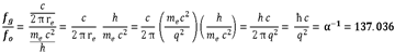
We present a novel approach which unveils its primordial physical origin, which has not been reported so far. It arises from the structural properties of the electron, specifically from its two structural frequencies: the oscillation frequency: fo = me c2 / h and the gyratory frequency: fg = c / 2 π re where re is the classical electron radius with value q2 / me c2 = 2.82 10-15 m. So, we obtain:
It turns out that the inverse value of the fine-structure constant α-1 corresponds to the ratio between these two structural frequencies of the electron.
Regarding the electron radius used in the formulation of the ratio fg / fo let us point out that, likewise for the Bohr atom in which its radius is obtained from the balance of the centrifugal and centripetal forces on the electron peripheric orbital, the structural radius of the electron can also be obtained from the balance of the centrifugal F↑ and centripetal F↓ forces on its structural carrier electric charge.
F↓ = q2 / re2and F↑ = me c2 / re
For F↓ = F↑ we get: q2 / re2 = me c2 / re
So, re = q2 / me c2
The standard semi-classical formulation of the electron magnetic moment is:
μe = ½ q ћ / me
However, it can also be expressed rearranging the above formulation so that the inverse fine-structure constant α-1 is introduced.
μe = ½ q ћ / me = ½ (ћ c / q2) q c (q2 / me c2) = ½ α-1 q c re
where re = q2 / me c2. Applying the classical expression of re we obtain:
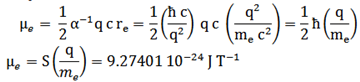
S being the electron spin ћ/2 and q/me its so-called charge-to-mass ratio of value 1.76 1011 C/kg.
It turns out that to obtain the value of the electron’s magnetic moment 23, 24, 25, its classical formulation μ = ½ q v r must be multiplied by the reciprocal fine-structure constant α-1 and v equated to c, which means that the orbital speed of its structural carrier electric charge is equal to the speed of light. This is possible due to the fact that the electric charge is massless. Furthermore, we must wonder why the classical formulation of the electron’s magnetic moment must be increased by the reciprocal fine-structure constant. To do this, let us define two fundamental characteristics of the electron’s structure, specifically its structural gyratory frequency and its oscillatory frequency, and express their ratio.
fg = c / 2 π re →fg = 1.6932 1022 Hz
where re stands for the classical expression q2/ me c2 of the electron radius.
fo = me c2 / h→fo = 1.23559 1020 Hz
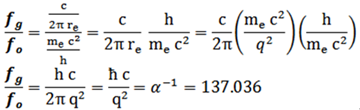
fg / fo = (c / 2 π re) / (me c2 / h) = (me c3 / 2 π q2) / (me c2 / 2 π ћ) = ћ c / q2 = α-1 = 137.036
fg / fo = α-1
It emerges that the ratio fg / fo is precisely equal to the reciprocal fine-structure constant α-1. Therefore, to obtain the electron’s magnetic moment, the classical formulation must be amended by adding the ratio of its two structural frequencies, as a relevant influential factor determining its value. The fact that fg / fo = α-1 = 137.036 means that, within the time span of one oscillation of the electron’s structural electric charge, it has done 137.036 rotations.
µ = ½ α-1 q c re = ½ (fg / fo) q c re since:fg / fo = α-1
Thus, the electron’s magnetic moment is determined by the number of rotations of its structural electric charge during the time span of one oscillation, which acts as the referential unit of time. This means that the electron’s magnetic moment is not governed by the number of rotations per second of its structural electric charge, but by the number of rotations per time span of one period T, which acts as the effective unit of time, justifying the factor α-1 in the formulation of the electron’s magnetic moment 26, 27, 28. This highlights that, at the Fermi scale (10-15 m), the structural frequencies of elementary particles must be taken into account when defining some of their characteristics, as in the case for the muon’s magnetic moment.
In other words, to obtain the electron’s magnetic moment, the classical formulation should be multiplied by the fg / fo ratio. The oscillatory frequency fo acts as a kinematic reference unit, so the classical value of μe must be multiplied by 137.036, which is the number of rotations that the structural electric charge of the electron makes during the time span of one oscillation.
µ = ½ (fg / fo) q c re
where fg = c / 2 π re fo =me c2 / h re = q2 / me c2
µ = ½ (c / 2π re) / (me c2 / h) q c re = ½ (ћ / c) (q / me) = ½ ћ q / me
Consequently, it arises that the electron’s magnetic moment is determined by the ratio fg / fo of its two structural frequencies.
Actually, the electron’s magnetic moment is slightly higher than the calculated value, the experimental value of which is 9.28476469173 10-24 J T-1, requiring a corrective factor known as the g-factor 28, 31, with a value of 1.00116. It is worth mentioning that, like the ratio fg / fo of the structural gyratory frequency and oscillatory frequency of the electron, its corrective gfactor can also be expressed in terms of the fine-structure constant:
ge = 1+1/(2π α) = 1+1/[2π (fg / fo)].
However, unlike the fg / fo factor, whose physical origin lies in the electron’s structural frequencies, the physical origin of the corrective gfactor is not explained in this context, since the electric charge interaction with the socalled quantum vacuum is not taken into account, as QED does.
Here, rather than aiming for the most precise numerical derivation of the electron’s magnetic moment, this approach prioritizes revealing the fundamental physical origin of the fine-structure constant as expressing the ratio fg / fo of the electron’s structural gyratory and oscillatory frequencies, and its fundamental role in various fields.
3.2. Relationship of the Structural Frequencies fg / fo to the Ratio re / ƛe of the Electron Classical Radius re and its associated Structural Wavelength ƛefo = c / λ = c / 2π ƛ → ƛe = c / 2π fo
and fg = c / 2π r → re = c / 2π fg
So: re / ƛe = (c / 2π fg) / (c / 2π fo) = (c / fg) / (c / fo)
= (c / fg) (fo / c) = fo / fg
Therefore, the equivalence between the ratios ƛe / re and fo / fg attests the factuality of the two structural frequencies of the electron since the gyratory frequency is related to its radius and the oscillatory frequency is related to its associated structural wavelength.
re = q2 / me c2ƛe = ћ / me c = ћ c / me c2thus:
ƛe / re = (ћ c / me c2) / (q2 / me c2) = ћ c / q2 = α-1
= 1 / 137.036 and:
fg / fo = (c / 2 π re) / (me c2 / h) = (me c3 / 2 π q2) / (me c2 / h)
= h c / 2 π q2 = ћ c / q2 = α-1 = 137.036
Since the ratio fg / fo is equal to the inverse fine-structure constant α-1, and the ratio ƛe / re of the electron’s associated wavelength and its classical radius is also equal to α-1, therefore ƛe / re = fg / fo .
Let us highlight that the electron’s wavelength does not derive from a kinetic energy due to its motion, but is instead an intrinsic wavelength resulting from its structural oscillatory frequency, which in turn defines its structural energy: E = h c / λ = h fo = me c2.
Equivalently to the ratio fg / fo of the gyratory frequency and the oscillatory frequency of the electron’s structural carrier, the inverse fine-structure constant can be expressed as the ratio ƛe / re of the classical electron radius and its associated wavelength, since fg is a function of re (fg = c / 2π re) and fo is a function of λ, since by definition f = c / λ.
re = q2 / me c2 and ƛe = ћ / me c = ћ c / me c2
α = re / ƛe = q2 / ћ c
3.3. Relationship of the Structural Frequencies fg / fo to the Ratio rH / re of the Bohr Atomic Radius rH and the Electron Classical Radius reThe Bohr radius is: rH = ћ2 / me q2 = 0.529 Angstroms = 0.529 10-10 m = 52. 9 pico-meter (1012 m)
The electron classical radius is: re = q2 / me c2 = 2.82 femto-meter (10-15 m).
So, rH / re = (ћ2 / me q2) / (q2 / me c2) = (ћ c / q2)2
rH / re = α-2 = (137.036)2 rH = α-2 re = (fg / fo)2 re
Therefore, the ground state radius of the H atom is (137.036)2 times larger than the electron classical radius. This does not seem to be a coincidence, and the electron radius is assumed to be related to the Bohr radius 32 of the hydrogen atom via the fine-structure constant.
Hence, the ground state radius of the H atom is a multiple of α-2 times the electron radius, but since α-1 = (fg / fo) it turns out that its radius is paired to the structural frequencies of the electron. This highlights the influence of the ratio fg / fo on the H atom radius since fg / fo is a property of the electron, and reveals that the H atom radius is coupled to the electron structural frequencies.
3.4. Relationship of the Electron’s Structural Frequencies fg / fo to the Ratio v / c of Neils Bohr’s Atomic Orbital ModelFor the peripheral electron to maintain a circular orbit, the Coulomb centripetal force it experiences due to the nucleus attraction must be equal to the centrifugal force due to the rotation of its structural electric charge:
F↓ = F↑
F↓ = q2/ r2 and F↑ = me v2 / r
F↓ = F↑ → rH = q2 / me v2
On its part, the momentum L of the peripheric electron is quantized with value ћ.
L = me v rH = ћ therefore: v = ћ / me rH
v = ћ / me rH = (ћ / me) (me v2 / q2) = q2 / ћ
thus: v / c = q2 / ћ c = α
and since: (fg / fo)-1 = α
therefore: v / c = (fg / fo)-1
The fact that v / c = (fg / fo)-1 = α = (137.036)-1 means that the velocity v of the peripheric electron of the H atom is coupled to the inverse ratio fg / fo of the structural frequencies of the electron, and that v is 137.036 times smaller than c.
In other words, the velocity v of the electron around the proton of the H atom is ruled by the ratio fg / fo of the two structural frequencies of the electron itself, such as v = c (fg / fo)-1. Therefore, it is the ratio fg / fo that induces the velocity of the orbital electron of the hydrogen atom, and it is shown below that it also governs other systems.
3.5. Relationship of the Electron Structural Frequencies fg / fo to the H Ground State Energy Level and the Electron Structural FrequenciesGround state energy of the Bohr model of the H atom:
E = T + V = ½ me v2 – q2 / rH = - ½ q2 / rH
where v = q2/ h is the velocity of the peripheric electron and rH = ћ2 / me q2 is the ground state radius of the H atom, thus: E0 = - ½ q2 / (ћ2 / me q2) = - ½ me (q4/ ћ2)
= - ½ me c2 (q4/ ћ2 c2) = - ½ me c2 (q2/ ћ c)2
E0 = - ½ α2 me c2
So, the ground state E0 of the H atom is a multiple of α-1 but since α = (fg / fo) -1 it turns out that its ground state is coupled to the structural frequencies of the electron.
E0 = - ½ α2 me c2 = - ½ (fg / fo)-2 me c2 = -13.6 eV
3.6. Ratio of the Muon Structural Frequencies fg / fo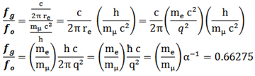
This displays that for the muon the ratio fg / fo is much smaller than that for the electron, which is instead equal to 137.036. This indicates that in the very short time span of one oscillation, the muon’s structural electric charge has not even completed one rotation. The classical radius of the muon is taken to be the same as that of the electron: rµ = re = q2 / me c2, since they differ only in their structural oscillatory frequency, the muon being no more than an excited oscillatory state of the electron that retains the same structural radius.
3.7. Relationship of the Muon Structural Frequencies fg / fo to its Magnetic Momentfo = mμ c2 / h→fo = 2.5548 1022 Hz
fg = c / 2 π rµ →fg = 1.6932 1022 Hz
where rµ is the muon classical radius: rμ = re = q2 / me c2 = 2.82 10-15 m which is the same radius as that of the electron, since the muon is seen as an excited oscillatory state of the electron, maintaining the same radius of their structural orbital.
fg / fo = (c / 2 π rμ) / (mμ c2 / h) = (me c3 / 2 π q2) / (mμ c2 / h) = (me / mμ) (ћ c / q2) = 0.66275
Tg = 1/fg = 5.9060 10-23 s
To = 1/fo = 3.9143 10-23 s
This means that it the time span of one oscillation (To) which lasts only 3.9 10-23 s the muon’s structural electric charge has completed only 0.66275 rotation, since one rotation takes a time (Tg) of 5.9 10-23 s.
The muon and the electron have the same gyratory frequency of their structural electric charge and differ only in their structural oscillatory frequency. The muon has a structural oscillatory frequency of 2.5548 1022 Hz, i.e. 206.768 times higher than that of the electron of only 1.23559 1020 Hz. This high oscillatory frequency of the muon structure is the origin of its high structural energy (E = h f ) and its correlated high mass (E = mμ c2).
Magnetic moment of the muon:
µµ = ½ (fg / fo) q c rµ= ½ α-1 (me / mμ) q c rµ = (me / mμ) µe = (0.511/ 105.66) µe = µe / 207
The muon’s small magnetic moment 33, 34 is due to the fact that the period of one oscillation (Tµ = 3.9143 1023 s) is almost 207 times shorter than that of the electron (Te = 8.0933 1021 s), so in such a short period of the muon’s structural oscillation, its vector electric charge has rotated much less (only 0.66 rotation) than in the case of the electron (137.036 rotations). Let us recall that, as for the electron, the oscillatory period acts as the unit of time that fixes the number of rotations of the structural electric charge in the corresponding time span, a fact that follows from the coupling between structural rotation and oscillation.
3.8. Predicted Value of the Tau Magnetic MomentLet us first calculate the tau structural oscillatory frequency and its gyratory frequency:
fo = mτ c2 / h = 4.2964276 1023 Hz
since: mτ = 3.16754 10-27 kg
fg = c / 2 π rτ = 1.6932031 1022 Hz
since: rτ = re = q2 / me c2 = 2.82 10-15 m
Let us justify the equality of the tau and electron radius. Just as the muon, the tau is considered to be an oscillatory excited state of the electron, in which the gyratory radius of the electron is preserved.
Applying the fg / fo ratio to the tau we obtain:
fg / fo = (c / 2 π rτ) / (mτ c2 / h) = (me c3 / 2 π q2) / (mτ c2 / h) = (me / mτ) (ћ c / q2) = α-1 (me / mτ) = 0.03941
This means that in the time span of one oscillation the structural electric charge of the tau has only made 0.03941 rotation. Applying this to the tau’s magnetic moment gives:
μτ = ½ (fg / fo) q c rτ = ½ ћ q / mτ = 2.66707 10-27 J /T
while the QED value is ≈ 2.67 10-27 J / T
This shows that our approach based on the fg / fo ratio and a semi-classical formalism does it as well as the QED, since in good agreement with the tau’s magnetic moment, and therefore proves the rightness of our procedure.
3.9. Ratio of the Electron Structural Frequencies fg / fo in Relation to the Rydberg Constant
Since R∞ = α2 / 2 λe and since λe = c / fo and α = fo / fg then: R∞ = fo (α2 / 2 c) = fo (fo / fg)2 / 2 c
The Rydberg constant appears thus to be a result of the structural characteristics of the electron itself, as it depends on its gyratory and oscillatory frequencies.
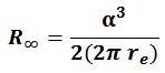
Furthermore, since R∞ is also expressed as:
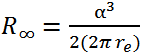
It is thus equivalent to:

Hence, from this formulation the Rydberg constant turns out to be the ratio of fo / fg raised to the third power and over twice the circumference of the electron structural orbital.
The formulation of R∞ containing the ratio fg / fo introduces hence a new approach to the Rydberg constant 35, 36, 37.
3.10. Relationship of the Electron Structural Frequencies fg / fo to other ApplicationsIn any electromagnetic formulation where the fine-structure constant α appears, it can be replaced by the ratio of the electron structural frequencies fg / fo since α originates from their ratio. This therefore demonstrates that the electromagnetism is governed by the ratio fg / fo of the electron structural frequencies.
Since the gyratory frequency fg = c /2 π r depends on the particle’s structural radius and the structural oscillatory frequency fo = m c2 / h depends on the particle’s mass, it appears obvious that the ratio fg / fo is equal to the inverse of the fine-structure constant α-1 only for the electron, and therefore fg / fo = α-1 is relevant only to electron-related applications. Logically, the coupling constant 38, 39 of the fundamental forces other than the electromagnetic force is therefore not equal to the fine-structure constant, being equal to 1 for the strong interaction, 10-6 for the weak interaction and 10-39 for the gravitational interaction.
We have shown that the properties of electron-based entities derive in first instance on the structural characteristics of the electron itself, specifically from the ratio fo / fg of its structural oscillatory and gyratory frequencies, the electron being a gyratory-oscillator. From the aforementioned applications, it follows that the fine-structure constant is indeed a constant in the sense that it arises specifically from the electron, expressing the ratio fo / fg of its two structural frequencies.
For the fine-structure constant not to be a constant would imply a shift of the electron’s properties over time, which is quite unlikely. Since it has been demonstrated that the physical origin of the fine-structure constant is rooted on the electron, this put in a difficult position those theories that forecast its variation over cosmic time 40, 41, 42, 43, 44, 45, 46, since it would imply the variation of the electron itself.
On experimental grounds diverse procedures have been achieved, such as atom recoil experiments, electron magnetic moment (g-2), polarization rotation in topological insulators, quantum hall effect and spectroscopy of hydrogen-like atoms. Each technique brings a different strength. Though, comparatively our approach presents the great advantage to focus on a most primordial element: the electron itself, and its structural properties. It should also be noted that the origin of the fine-structure constant is restricted to the electron and its excited states the muon and the tau, and does not apply to other particles, which ratio fo / fg has not the same assessment.
Our novel approach to the fine-structure constant has provided its primordial physical origin, from which all other derivations follow, since the electron is the centerpiece of electromagnetism. The semiclassical approach has proven highly efficient in uncovering the physical origin of the fine-structure constant, emerging from the electron. Demonstrating its primordial origin has been straightforward and no sophisticated mathematical approaches has been required. Therefore, before delving into complex mathematical approaches – where greater the complexity often leads to weaker physical grounding – it should first be assessed whether the semi-classical context is efficiently operative. This has the added advantage of offering a simple depiction of the physical foundation.
While quantum electrodynamics (QED) has been very productive in many areas, it has also been an hindrance in others. No theory is perfect or exhaustive, it is always just an approach to a physical description. Moreover, any theoretical framework may be replaced or may lose some of its appeal over time, but the underlying physical principles remain unchanged. In particular, QED’s rejection of the electron having an internal structure – based on a biased deduction from high-energy electron collisions – has inhibited the discovery of the primordial origin of the fine-structure constant, which is specifically rooted in the electron's structure.
The reason the fine-structure constant is a dimensionless quantity is simply that it expresses the ratio of two frequencies. Its physical value corresponds to 137.036 rotations of the electron’s structural electric charge within the time span of one oscillation. Thus, there is no longer any mystery regarding the fine-structure constant’s value and its dimensionless nature. It has been demonstrated that the electron possesses two structural frequencies, which establish the primordial origin of the fine-structure constant, and define some of its applications.
However, the equivalency between the fine-structure constant α and the ratio fg / fo of the electron’s gyratory and oscillatory structural frequencies is not always valid. It applies specifically to the electron and its related physical processes. Nevertheless, the ratio fg / fo can be extended to the muon and the tau, since they are considered excited states of the electron and thus their frequency ratio fg / fo can be respectively expressed as α-1 (me / mμ) and α-1 (me / mτ).
The primordial origin of the fine-structure constant has been identified as the electron itself, through its two structural frequencies – the gyratory and the oscillatory frequency of its structural carrier electric charge. The ratio fo / fg = α-1 – confirming that α is dimensionless since it expresses a ratio of two frequencies. With this understanding, we have answered two fundamental questions posed by the physics community: the primordial origin of the fine-structure constant and why it is dimensionless. Furthermore, it has been shown that the electron’s structural frequencies regulate the behavior of physical systems based on it.
The fine-structure constant extracted from the electron should be further explored in the realm of quantum mechanics. Here, the semi-classical approach has already proven that the fine-structure constant represents the ratio between the electron’s two structural frequencies, and it has been focused on demonstrating it pedagogically.
N.B.: In seek of making mathematical formulations simpler, the factor related to the permittivity of vacuum, necessary in order to get numerical values, has been omitted. The complete formulation of α and re are:
α1 = k-1 (ћ c / q2) and re = k (q2/ me c2) where k = 1/(4 π ε0) and ε0 is the permittivity of vacuum.
| [1] | Current advances: The fine-structure constant. | ||
| In article | |||
| [2] | Fine-structure constant – Wikipedia. | ||
| In article | |||
| [3] | Dupays, J. (2003) The Fine-Structure Constant: From Eddington's Time to the Present Contemporary Physics, 44(4), 319–331. | ||
| In article | |||
| [4] | Barrow, J. D. (2002) The Constants of Nature: From Alpha to Omega Vintage Books. | ||
| In article | View Article | ||
| [5] | Bouchendira, R. et al. (2011), New Determination of the Fine-Structure Constant, Physical Review Letters. | ||
| In article | View Article PubMed | ||
| [6] | Morel, L. et al. (2020). Determination of the Fine-Structure Constant with Rubidium Atoms, Nature. | ||
| In article | |||
| [7] | Evaluation of the Fine Structure Constant Adriano Alippi, Journal of Modern Physics Vol.11 No.12, December 7, 2020. | ||
| In article | View Article | ||
| [8] | Calculation of the Fine-Structure Constant, Jesús Sánchez, Journal of High Energy Physics, Gravitation and Cosmology > Vol.4 No.3, July 2018. | ||
| In article | |||
| [9] | Bohr model – Wikipedia. | ||
| In article | |||
| [10] | Sommerfeld, A. (1916) Zur Feinstruktur der Wasserstofflinien (On the Fine Structure of Hydrogen Lines) - Annalen der Physik, 51(17), 1–94. | ||
| In article | View Article | ||
| [11] | Bohr–Sommerfeld model – Wikipedia. | ||
| In article | |||
| [12] | Schrödinger Equation for the Hydrogen Atom.pdf. | ||
| In article | |||
| [13] | 4.10: The Schrödinger Wave Equation for the Hydrogen Atom - Chemistry Libre Texts. | ||
| In article | |||
| [14] | Schröder's equation – Wikipedia. | ||
| In article | |||
| [15] | J. S. Schwinger, On quantum electrodynamics and the magnetic moment of the electron, Phys. Rev. 73, 416 (1948). | ||
| In article | View Article | ||
| [16] | Introduction to the Dirac Equation (2020) Robert G. Littlejohn dirac.dvi. | ||
| In article | |||
| [17] | Dirac equation – Wikipedia. | ||
| In article | |||
| [18] | P. A. M. Dirac, The quantum theory of electron. Part II, Proc. R. Soc. A 118, 351 (1928)(PDF) The Quantum Theory of the Electron. Part II (1928) | Paul Adrien Maurice Dirac |. | ||
| In article | View Article | ||
| [19] | Quantum Electrodynamics (QED)Quantum electrodynamics – Wikipedia. | ||
| In article | |||
| [20] | https://www.damtp.cam.ac.uk/user/tong/qft/six.pdf. | ||
| In article | |||
| [21] | Quantum electrodynamics – Wikipedia. | ||
| In article | |||
| [22] | S.M. Blinder - Structure and Self-Energy of the Electron https://deepblue.lib.umich.edu/bitstream/handle/2027.42/34397/1806_ftp.pdf?sequence=1. | ||
| In article | |||
| [23] | Electron – Wikipedia. | ||
| In article | |||
| [24] | 8.3: Orbital Magnetic Dipole Moment of the Electron - Physics Libre Texts. | ||
| In article | |||
| [25] | Electron magnetic moment - Wikipedia. | ||
| In article | |||
| [26] | Electron anomalous magnetic moment: history and current status | ||
| In article | |||
| [27] | New Measurement of the Electron Magnetic Moment and the Fine Structure Constant, D. Hanneke, S. Fogwell, and G. Gabrielse - Physical Review Letters (2008), https:// cfp. physics.northwestern.edu/ documents/ Harvard Electron Magnetic Moment2008.pdf. | ||
| In article | |||
| [28] | Electron Magnetic Moment. | ||
| In article | |||
| [29] | Anomalous magnetic dipole moment – Wikipedia. | ||
| In article | |||
| [30] | g-factor (physics). | ||
| In article | |||
| [31] | g-factor (physics) – Wikipedia. | ||
| In article | |||
| [32] | Gabrielse, G. et al. (2006) New Determination of the Fine-Structure Constant from the Electron g-Value and QED, Physical Review Letters, 97(3): 030802. | ||
| In article | View Article PubMed | ||
| [33] | Bohr radius – Wikipedia. | ||
| In article | |||
| [34] | Muon g − 2: A review – ScienceDirect. | ||
| In article | |||
| [35] | Muon g − 2 Collaboration Phys. Rev. Lett. 126, 141801 (2021) | ||
| In article | |||
| [36] | Rydberg constant | Definition, Formula, Value, & Facts | Britannica. | ||
| In article | |||
| [37] | Rydberg constant – Wikipedia. | ||
| In article | |||
| [38] | CODATA Value: Rydberg constant. | ||
| In article | |||
| [39] | Coupling Constants for the Fundamental Forces. | ||
| In article | |||
| [40] | https://en.wikipedia.org/wiki/Coupling_constant. | ||
| In article | |||
| [41] | Uzan, J.-P. (2003) The Fundamental Constants and Their Variation: Observational and Theoretical Status, Reviews of Modern Physics, 75(2): 403–455. | ||
| In article | View Article | ||
| [42] | Parker, R. H., et al. (2018), Measurement of the Fine-Structure Constant as a Test of the Standard Model. Science, 360 (6385), 191–195. | ||
| In article | View Article PubMed | ||
| [43] | Kinoshita, T. (2006). The Fine-Structure Constant and Quantum Electrodynamics, Reports on Progress in Physics, 69(8), 2443–2504. | ||
| In article | |||
| [44] | Duff, M. J. (2015). How Fundamental Are Fundamental Constants? Contemporary Physics, 56(1), 35–47. | ||
| In article | View Article | ||
| [45] | (PDF) New Constraints on variations of the fine structure constant from CMB anisotropies. | ||
| In article | |||
| [46] | Webb, J. K. et al. (1999) Search for Time Variation of the Fine-Structure Constant Physical Review Letters, 82(5): 884–887. | ||
| In article | View Article | ||
Published with license by Science and Education Publishing, Copyright © 2025 G. Sardin
![]() This work is licensed under a Creative Commons Attribution 4.0 International License. To view a copy of this license, visit
http://creativecommons.org/licenses/by/4.0/
This work is licensed under a Creative Commons Attribution 4.0 International License. To view a copy of this license, visit
http://creativecommons.org/licenses/by/4.0/
| [1] | Current advances: The fine-structure constant. | ||
| In article | |||
| [2] | Fine-structure constant – Wikipedia. | ||
| In article | |||
| [3] | Dupays, J. (2003) The Fine-Structure Constant: From Eddington's Time to the Present Contemporary Physics, 44(4), 319–331. | ||
| In article | |||
| [4] | Barrow, J. D. (2002) The Constants of Nature: From Alpha to Omega Vintage Books. | ||
| In article | View Article | ||
| [5] | Bouchendira, R. et al. (2011), New Determination of the Fine-Structure Constant, Physical Review Letters. | ||
| In article | View Article PubMed | ||
| [6] | Morel, L. et al. (2020). Determination of the Fine-Structure Constant with Rubidium Atoms, Nature. | ||
| In article | |||
| [7] | Evaluation of the Fine Structure Constant Adriano Alippi, Journal of Modern Physics Vol.11 No.12, December 7, 2020. | ||
| In article | View Article | ||
| [8] | Calculation of the Fine-Structure Constant, Jesús Sánchez, Journal of High Energy Physics, Gravitation and Cosmology > Vol.4 No.3, July 2018. | ||
| In article | |||
| [9] | Bohr model – Wikipedia. | ||
| In article | |||
| [10] | Sommerfeld, A. (1916) Zur Feinstruktur der Wasserstofflinien (On the Fine Structure of Hydrogen Lines) - Annalen der Physik, 51(17), 1–94. | ||
| In article | View Article | ||
| [11] | Bohr–Sommerfeld model – Wikipedia. | ||
| In article | |||
| [12] | Schrödinger Equation for the Hydrogen Atom.pdf. | ||
| In article | |||
| [13] | 4.10: The Schrödinger Wave Equation for the Hydrogen Atom - Chemistry Libre Texts. | ||
| In article | |||
| [14] | Schröder's equation – Wikipedia. | ||
| In article | |||
| [15] | J. S. Schwinger, On quantum electrodynamics and the magnetic moment of the electron, Phys. Rev. 73, 416 (1948). | ||
| In article | View Article | ||
| [16] | Introduction to the Dirac Equation (2020) Robert G. Littlejohn dirac.dvi. | ||
| In article | |||
| [17] | Dirac equation – Wikipedia. | ||
| In article | |||
| [18] | P. A. M. Dirac, The quantum theory of electron. Part II, Proc. R. Soc. A 118, 351 (1928)(PDF) The Quantum Theory of the Electron. Part II (1928) | Paul Adrien Maurice Dirac |. | ||
| In article | View Article | ||
| [19] | Quantum Electrodynamics (QED)Quantum electrodynamics – Wikipedia. | ||
| In article | |||
| [20] | https://www.damtp.cam.ac.uk/user/tong/qft/six.pdf. | ||
| In article | |||
| [21] | Quantum electrodynamics – Wikipedia. | ||
| In article | |||
| [22] | S.M. Blinder - Structure and Self-Energy of the Electron https://deepblue.lib.umich.edu/bitstream/handle/2027.42/34397/1806_ftp.pdf?sequence=1. | ||
| In article | |||
| [23] | Electron – Wikipedia. | ||
| In article | |||
| [24] | 8.3: Orbital Magnetic Dipole Moment of the Electron - Physics Libre Texts. | ||
| In article | |||
| [25] | Electron magnetic moment - Wikipedia. | ||
| In article | |||
| [26] | Electron anomalous magnetic moment: history and current status | ||
| In article | |||
| [27] | New Measurement of the Electron Magnetic Moment and the Fine Structure Constant, D. Hanneke, S. Fogwell, and G. Gabrielse - Physical Review Letters (2008), https:// cfp. physics.northwestern.edu/ documents/ Harvard Electron Magnetic Moment2008.pdf. | ||
| In article | |||
| [28] | Electron Magnetic Moment. | ||
| In article | |||
| [29] | Anomalous magnetic dipole moment – Wikipedia. | ||
| In article | |||
| [30] | g-factor (physics). | ||
| In article | |||
| [31] | g-factor (physics) – Wikipedia. | ||
| In article | |||
| [32] | Gabrielse, G. et al. (2006) New Determination of the Fine-Structure Constant from the Electron g-Value and QED, Physical Review Letters, 97(3): 030802. | ||
| In article | View Article PubMed | ||
| [33] | Bohr radius – Wikipedia. | ||
| In article | |||
| [34] | Muon g − 2: A review – ScienceDirect. | ||
| In article | |||
| [35] | Muon g − 2 Collaboration Phys. Rev. Lett. 126, 141801 (2021) | ||
| In article | |||
| [36] | Rydberg constant | Definition, Formula, Value, & Facts | Britannica. | ||
| In article | |||
| [37] | Rydberg constant – Wikipedia. | ||
| In article | |||
| [38] | CODATA Value: Rydberg constant. | ||
| In article | |||
| [39] | Coupling Constants for the Fundamental Forces. | ||
| In article | |||
| [40] | https://en.wikipedia.org/wiki/Coupling_constant. | ||
| In article | |||
| [41] | Uzan, J.-P. (2003) The Fundamental Constants and Their Variation: Observational and Theoretical Status, Reviews of Modern Physics, 75(2): 403–455. | ||
| In article | View Article | ||
| [42] | Parker, R. H., et al. (2018), Measurement of the Fine-Structure Constant as a Test of the Standard Model. Science, 360 (6385), 191–195. | ||
| In article | View Article PubMed | ||
| [43] | Kinoshita, T. (2006). The Fine-Structure Constant and Quantum Electrodynamics, Reports on Progress in Physics, 69(8), 2443–2504. | ||
| In article | |||
| [44] | Duff, M. J. (2015). How Fundamental Are Fundamental Constants? Contemporary Physics, 56(1), 35–47. | ||
| In article | View Article | ||
| [45] | (PDF) New Constraints on variations of the fine structure constant from CMB anisotropies. | ||
| In article | |||
| [46] | Webb, J. K. et al. (1999) Search for Time Variation of the Fine-Structure Constant Physical Review Letters, 82(5): 884–887. | ||
| In article | View Article | ||