It is presented a code using a free software in order to calculate optical parameters for an arbitrary system consisting in N thick lenses submerged in optical media with arbitrary refraction index. This code calculates focus, front and back focal distances, principal planes and image distances for such multi-lens systems. The software was verified by solving numeric examples extracted from well-established optics literature.
Resolving optical multi-lenses systems can be very laborious if doing by hand. There exists commercial software up to the task and of professional level to perform such assignment 1, 2. They have their correspondent educational free versions, but their code is obviously hidden, and in some cases are far from been user friendly, especially for the beginner optic student. In this paper, as a way of complementing this picture, it is presented an algorithm using an open-source software, Scilab 3, which can be used to calculate some basic optical parameters such as focus, principal planes, front and back focal distances and the image distance (given the object distance), for an optical system composed by ‘N’ spherical thick lenses in cascade merged in N+1 optical media with arbitrary values of index of refraction. This algorism was verified by solving several numeric examples from publications and text books.
The main objective of this work is to present to the community, a free source code that eventually could be improved in order to perform also more sophisticated task, such as finding pupils, windows, field of view, estimating local of apertures, stops, and the likes. The algorithm that it is presented works for complex optical systems from two thick lenses onwards, and also can be used for the most idealized case of thin lenses.
The routine was implemented using Scilab and is based on the optical matrix method, assuming paraxial approximation, whose complete formalism is described in detail in 4. The aim is to resolve an optical system as shown in the Figure 1:

The optical system consists in an arbitrary number of ‘N’ spherical thick lenses (being N >1), each one with its glass of specified indices of refraction, na, nb,…nN, thicknesses, da, db,…dN, and radius, R1a, R2a,…R1N, R2N, immersed in optical media with dissimilar indices of refraction, n1, n2,…nN+1, and separated by distances dab, dbc,…dN-1,N. The horizontal line crossing the center of each lens is the optical axis. The object distance, so, is measured with respect to the vertex point ‘V1a’, which is the intersection of the first surface of the first lens with the optical axis. The image distance, si, is measured with respect to the vertex point ‘V2N’, which is the intersection of the second surface of the last lens with the optical axis. Regarding signal convention; object distances will be positive (negative) if the object is to the left (right) of ‘V1’, image distances will be positive (negative) if the image is to the right (left) of ‘V2N’. Concerning the curvature radii of surfaces, they will be positive (negative) if the corresponding surface was convex (concave). This convention is usually adopted in most of the specialized literature.
The idea is to calculate, for the complex system shown in Figure 1, the focal distance, f (also known as effective focal distance in some texts); the front focal distance, zf, that is the distance, measure from ‘V1a’ on the optical axis, in which an object point (or a source of spherical divergent wave fronts), must be located in order that the optical system produces a bunch of parallel rays after refraction (see Figure 2 the red rays); back focal distance, zb, which is the distance, measured from ‘V2N’, to which the optical system focalizes a bunch of optical ray incident parallel to the optical axis (see the blue rays Figure 2).

Front focal point, zf, related to front focal distance obeys the following signal convention; if positive, it should be located to the left of ‘V1a’, if negative, it should be localized to the right of ‘V1a’. For back focal point, zb, the following signal convention should be applied; if positive (negative), it should be localized to the right (left) of ‘V2N’.
Also, there will be calculated the two principal planes, 1PP and 2PP, whose distances, h1 and h2 are measured with respect to the already defined outermost vertex points of the system, ‘V1a’ and ’V2N’. Distance h1 obeys the following signal convention: if positive (negative), it is located to the right (left) of ‘V1a’. For h2 being positive (negative), h2 must be located to the right (left) of ‘V2N’. These planes are useful in order to simplify the object-image equation for such a complicated system. Also are shown in Figure 2, the quantities so´ and si´, which are object and image distances with respect to the principal planes, respectively. These auxiliary distances are actually those that allow on to describe the optical system through a simple Gaussian type equation. For more details about these cardinal points and the complete analysis of the optical system, the interested reader is referred to 4.
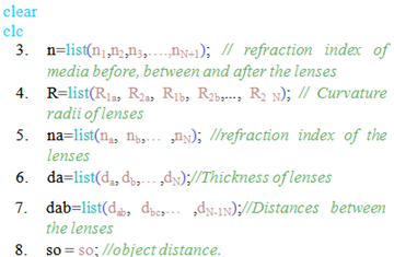
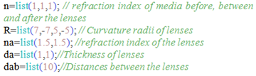
In this section is presented the code used to perform the calculations. The first lines consist in the input data for the system:
|
All data, except the object distance, are gathered using the “list” command. The line ‘n’ corresponds to the index of refraction of the media surrounding all lenses in order, i.e., the first, ‘n1’, corresponds to the first index of refraction medium before (to the left of) the first lens, the second, ‘n2’, corresponds to the index of refraction medium between first and second lenses, etc., until the last one, ‘nN+1’, (being N the total number of lenses), corresponds to the index of refraction of the optical medium after (to the right of) the last lens. The fourth line, `R´, gathers the radii of curvature of the lenses. The subindex `1a´, stands for the radius of the first surface of the first lens, subindex `2b´ for the radius of the second surface of the second lens, etc. In case there is a plane surface for some lens, the number `1e20´ will suffice as the value of an “infinite” radius. The line ‘na’ gathers the index of refraction values for each of the lenses compounding the system. The ‘da’ line gathers the thickness of each lens and finally, the ‘dab’ line should be filled with the correspondent distances between the lenses.
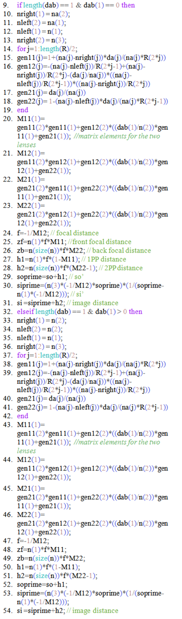
The next lines show the calculation for the specific case of two lenses:
|
The variables “genij” in lines 15-18 are the matrix elements for the individual lenses, for which, in addition to the index of refraction of the lenses themselves, the index of refraction of the media surrounding them, and eventually those of the adjacent lenses (in case the distances between them are null), are used. For that case, the lines 10-13 define the index accordingly. Then, in lines 15-18 the matrix elements are effectively calculated. After that, in lines 20-23 the matrix elements Mij for the two lenses systems are calculated. Finally in lines 24-31 the cardinal points and the image distance are calculated.
The lines 32-54 make the same calculation for the two lenses systems when the distance between them is not null.
The following lines perform the calculation for optical systems with more than two lenses:
|
The code was tested using three examples solved in the literature.
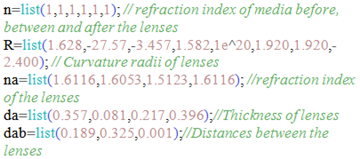
4.1. Example 1The first of them is the Tessar lens shown in 5, pages 250-251. The input data are filled as follows:
|
In the last line, i.e., distance between lenses, in order to reproduce the results it was necessary to simulate a thin air layer between the last two lenses, which seems reasonable from the figure of the Tessar shown in the aforementioned reference. The results obtained once the code was run (that can be accessed via variable navigator on Scilab Menu), are:
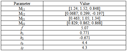
The first four lines show the successive values of the Mij matrices elements for the system analyzed in this example, calculated iteratively as shown by the lines ‘77-80’ of the code, for the two first lenses, and then by lines 81-85, for the rest of the system. The last figure in each line is the corresponding matrix element of the system, and the optical matrix corresponding to the Tessar lens is:
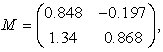 |
which is in very good agreement to the result presented in 5. Also, the values for the focal distance, f = 5.07 and the location of principal planes, h1 = 0.771 and h2 = -0.671, are in very good agreement with the results of that book. The units of the cardinal points are the same units of length of radii of curvature of the lens’s surfaces, which, of course, should be the same as that of the lens thicknesses.
4.2. Example 2The next example is from reference 6, where several complex geometric optics systems are analyzed. The first of them presented here is the numerical example 2 of such reference, where a two lenses system is evaluated. The data input lines for such example are:
|
In the next table the results obtained for this example in the reference are shown and compared with the values obtained using the software:
Note that nomenclature for the optical parameters is different, but the physical meaning is the same.
4.3. Example 3The next case corresponds to the numerical example 4 of the same reference, which consists in a five thick lenses system in between several optical index media, some of them different from air. The input data lines that reproduce such example are:
|
In Table 3 a comparative analysis between the results is shown.
Once more the agreement is excellent.
In the examples verified, there has not been used the line corresponding to object distance (in order to calculate image distance). This feature was corroborated using other examples. Also, the software can be used for the idealized case of thin lenses, writing simply da = 0, in the corresponding lenses.
In this work, it was presented a free code that calculates basic optical parameters such as focal distance, back and front focal distances, and principal planes, for a complex optical system composed of an arbitrary (minimum two) number of thick lenses surrounded by arbitrary refraction index´s optical media. Also, it can be used for calculation of image distance, given the object distance for this system. In addition, idealized cases of multiple thin lenses can also be studied.
| [1] | https://lambdares.com/oslo/ .[Accessed June. 04, 2023] | ||
| In article | |||
| [2] | https://www.zemax.com/. [Accessed June. 04, 2023] | ||
| In article | |||
| [3] | https://www.scilab.org/. [Accessed June. 04, 2023] | ||
| In article | |||
| [4] | Fulvio Andres Callegari. Thick Lenses Systems between Arbitrary Index of Refraction Optical Media. A Simple Optical Model for the Human Eye. International Journal of Physics, Vol. 9, No. 6, 2021, pp 259-268. Available: http://pubs.sciepub.com/ijp/9/6/1. [Accessed June. 04, 2023] | ||
| In article | View Article | ||
| [5] | Hecth, E, Optics, 4ed, Addilson Wesley, San Francisco, 2002, 250-251. | ||
| In article | |||
| [6] | Hassan A. Elagha, "Determination of the effective focal length and cardinal points for a coaxial system of thick lenses," Appl. Opt. 61, 6778-6786 (2022). | ||
| In article | View Article PubMed | ||
Published with license by Science and Education Publishing, Copyright © 2023 Fulvio Andres Callegari
![]() This work is licensed under a Creative Commons Attribution 4.0 International License. To view a copy of this license, visit
http://creativecommons.org/licenses/by/4.0/
This work is licensed under a Creative Commons Attribution 4.0 International License. To view a copy of this license, visit
http://creativecommons.org/licenses/by/4.0/
| [1] | https://lambdares.com/oslo/ .[Accessed June. 04, 2023] | ||
| In article | |||
| [2] | https://www.zemax.com/. [Accessed June. 04, 2023] | ||
| In article | |||
| [3] | https://www.scilab.org/. [Accessed June. 04, 2023] | ||
| In article | |||
| [4] | Fulvio Andres Callegari. Thick Lenses Systems between Arbitrary Index of Refraction Optical Media. A Simple Optical Model for the Human Eye. International Journal of Physics, Vol. 9, No. 6, 2021, pp 259-268. Available: http://pubs.sciepub.com/ijp/9/6/1. [Accessed June. 04, 2023] | ||
| In article | View Article | ||
| [5] | Hecth, E, Optics, 4ed, Addilson Wesley, San Francisco, 2002, 250-251. | ||
| In article | |||
| [6] | Hassan A. Elagha, "Determination of the effective focal length and cardinal points for a coaxial system of thick lenses," Appl. Opt. 61, 6778-6786 (2022). | ||
| In article | View Article PubMed | ||


