1. Introduction

Image compression has always been an important aspect of efficiently saving computerized memory. Data compression was first introduced in 1838 in the form of Morse code for telegraphy ^[1]. It was not until the development of information theory in the 1940s where numerous techniques in data compression were introduced to the world ^[1]. Many of these techniques were eventually applied towards images, videos, audio and several other areas where it became an asset. By observing specific differentiations between compression methods, it may be possible to pinpoint what causes a method of compression to produce higher compression ratio hence saving more space. Our team focused on mean manipulation to be one of the possible solutions of achieving higher compression ratios. We used two algorithms based on arithmetic and geometric mean formulations to find this solution. By experimenting on these distinct algorithms, we could inevitably determine which mean produces the greater compression ratio.

2. Background Information

Image compression is the process of reducing the amount of memory an image file requires on a device. Images are made of small elements of color as illustrated in Figure 1. Each pixel takes up memory in the form of a unit of cyber information known as bytes ^[2]. Thousands of pixels comprise a typical image, resulting in higher demands of storage space ranging from kilobytes (1000 bytes) to megabytes (1000 kilobytes); Table 1 shows the chain of sequence associated with the maximization of digital data. Both clarity and sharpness of an image is affected by the size and amount of pixels it encapsulates.

Figure 1. Video Compression and Decompression

Download as

PowerPoint Slide

Larger image(png format)

Figures index

Veiw figure

View current figure in a new window

View next figure

Image compression is used in a wide variety of multi-media devices including digital cameras, computers, smart phones, and several peripheral devices ^[3]; Figure 2 shows how compression and decompression occurs in a digital camera ^[4]. The compression of imagery is categorized into two distinct categories: lossless and lossy compression. In lossless compression, every single bit of data that was originally present in the file remains after the file is compressed; all of the information is completely restored. This is generally the technique of choice for financial spreadsheets and medical imagery, where losing the slightest amount of information may be critical and problematic. As opposed to lossless compression, lossy compression reduces a file by permanently eliminating certain information, which is usually redundant ^[3]. When the file is compressed, only a part of the original information still exists, although this cannot be detected by human senses. Lossy compression is generally used for video and audio, where a certain amount of information loss may not be detected by most users.

Table 1. Decimal values for standard units of digital information

Download as

PowerPoint Slide

Larger image(png format)

Tables index

Veiw figure

View current table in a new window

There are several methods of compressing image files. During the process of saving a file onto a computer, an individual has the choice of choosing from several options. Some of the most common methods of compression include JPEG (Joint Photographic Experts Group), GIF (Graphics Interchange Format), PNG (Portable Network Graphics), TIF (Tagged Image File Format), and RAW (Raw Image Formats).

The JPEG image file, commonly used for photographs and other complex images on the internet, is a method that uses lossy compression. Using JPEG compression, the user can decide how much loss to introduce, making a trade-off between file size and image quality ^[5]. JPEG does not work well on line drawings, lettering or simple graphics because there is not a lot of the image that can be eliminated in the lossy process, so the image loses clarity and sharpness ^[6].

Figure 2. Video Compression and Decompression

Download as

PowerPoint Slide

Larger image(png format)

Figures index

Veiw figure

View current figure in a new window

View previous figure

View next figure

Unlike JPEG, the GIF format is a lossless compression technique that supports only 256 colors. Generally, GIF is preferred over JPEG for images with only a few distinct colors, such as line drawings, black and white images and small texts that are only a few pixels large. With an animation editor, GIF images can be put together for animated images. GIF also supports transparency, where the background color can be set to transparent in order to let the color on the underlying Web page to show through ^[6].

As technology rapidly advances, it is important for computerized images to maintain their quality even after compression. Compression is really just a mathematical algorithm that is applied to an image’s content, and as such, altering these algorithms could significantly improve image compression.

3. Relevance

Image compression minimizes the timeit takes a webpage to load an image file. It also allowsfor the efficient use of bandwidth by providing high-quality images with a fraction of their original file sizes ^[7] .

Image compression is also important for the transmission of email attachments from one computer to another. Generally, it takes a longer time to load and retrieve the data when large file sizes are sent through emails as compared to smaller file sizes.

Similary, people who save large amounts of images onto hard drives, flash drives, or memory cardscould greatly benefit from image compression; by compressing imagesprior to them being saved, there will be more storage spacein a memory bank,and thus the user will save money without having to purchase a larger storage space.

Figure 3. RGB color wheel

Download as

PowerPoint Slide

Larger image(png format)

Figures index

Veiw figure

View current figure in a new window

View previous figure

View next figure

NASA is one of the many administations that strives to developefficient and effective compression processes. NASA uses their own personally designed compression method known as ICER to compress imagery. ICER is a progressive image compressor that can provide both lossless and lossy compression, and incorporates an error containment scheme to limit the effectsof data loss during transmission. It is a progressive compressionmechanism because as more compressed data is received, higher quality of reconstructed images can be reproduced ^[8].

On a daily basis, NASA receives millions of bytes of data which requires a large storage bank. Additionally, they have multiple backups for all the data they acquire. Compression saves NASA an enormous amount of hard drive space. Likewise, image andvideo compression saves transmission time ^[9]. NASA’sMars rovers sends back pictures and data which can take several months to reach Earth due to the massive distance between the two planets. To reduce this large transmission time, the rovers are equipped with a compression mechanism which compresses the information prior to being sent.

4. Mathematica Lab Experiment

Prior to conducting the experiment, a hypothesis was developed comparing the arithmetic and geometric means in addition to matrix variations: 2x2, 1x4, and 2x3. The team compressed ten images from five different categories: Venus, Earth, Mars, Jupiter, and Saturn. The team hypothesized that:

•  The geometric mean compression mechanism would save less space than arithmetic mean compression.

•  An image that is compressed by a 2x3 matrix will save more space than one that is compressed by fewer pixels, such as a 1x4 and 2x2 matrix.

•  An image compressed by a 2x2 matrix and 1x4 matrix will save the same amount of space; the orientation of the matrix does not affect the amount of space that is saved.

•  The compression ratio is unaffected by the different image categories (Venus, Earth, Mars, Jupiter, Saturn).

The arithmetic mean is defined as the sum of all numbers in a collection divided by the number of terms in the collection. The geometric mean is the nth root of the product of then numbers in a collection.

Formula for Arithmetic Mean:

Formula for Geometric Mean:

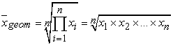Image compression can be pursued through a variety of mechanisms. For example, SVD compression uses singular value decomposition of matrices to reduce the amount of information stored in an image so that the image will occupy less space on a computer’s hard drive. Another compression mechanism may partition any given image into a variety of matrices of pixels. Each pixel has three numerical values between 0 and 1 representing the color of the pixel in red, green, and blue shades; the combination of these three colors forms every single color in the spectrum, as shown by Figure 3. The average values of the pixels within a partition can be taken and substituted for the original pixels.

In this experiment, the team used Wolfram Mathematica to find the most efficient means of compression ^[10]. More specifically, we used the arithmetic and geometric means to compress images to understand which mechanism saved more space. Within these broad mechanisms of compression, the team partitioned each image into three different matrices: 2x2, 1x4, and 2x3. Each image used in this experiment belonged to one of five categories: Earth, Venus, Mars, Jupiter, and Saturn. The team analyzed ten images from each category. Figure 4 is one of the selected images of Mars, which we used during the experimental process.

Figure 4. Surface of Mars

Download as

PowerPoint Slide

Larger image(png format)

Figures index

Veiw figure

View current figure in a new window

View previous figure

View next figure

Figure 5. Color channel separation

Download as

PowerPoint Slide

Larger image(png format)

Figures index

Veiw figure

View current figure in a new window

View previous figure

View next figure

Our Mathematica code first separated the image into three color channels: red, green, and blue, as indicated in Figure 5.

Each of the three images was then converted into a matrix; images are represented as matrices within computers because it is the only way that a computer is able to manipulate and store the data. We then set the dimensions, the width and length, of the desired variation – the size of the matrices each of the three images will be partitioned into. Next, our code added an infinite number of zeros to the right and below each of the three images to account for partitioning by a variation that does not divide the dimensions of the original image. It should be noted that adding zeros does not alter the content of the image in any respect.

Figure 6. Arithmetic mean compression for a 2x2 variation

Download as

PowerPoint Slide

Larger image(png format)

Figures index

Veiw figure

View current figure in a new window

View previous figure

View next figure

The numerical values in each partition within the three images are then averaged by the arithmetic mean. The average of each partition replaces the original values, as shown by Figure 6. After each of the three color channels is compressed by the arithmetic mean and the desired variation (i.e., a 2x2, 1x4 or 2x3 matrix), the three compressed color channels are combined, yielding a compressed version of the original image. For the geometric mean compression mechanism, images were compressed in the same manner hitherto mentioned with one exception: instead of taking the arithmetic mean of the numerical values in a partition, the geometric mean of the values was taken and substituted for the original values.

To find the most efficient means of compression, the team looked at average compression ratios. A compression ratio per image is defined as the file size of the original image divided by the file size of the compressed image. For each of the ten images in a category, the compression ratio was determined. The team then averaged the ten compression ratios to obtain the average compression ratio for a given category. The average compression ratio of each category was compared, as displayed by Figure 8 – Figure 12.

Figure 7. Full compression process

Download as

PowerPoint Slide

Larger image(png format)

Figures index

Veiw figure

View current figure in a new window

View previous figure

View next figure

Figure 8. categories vs. average compression ratio for a 2x2 partition size

Download as

PowerPoint Slide

Larger image(png format)

Figures index

Veiw figure

View current figure in a new window

View previous figure

View next figure

Figure 9. categories vs. average compression ratio for a 1x4 partition size

Download as

PowerPoint Slide

Larger image(png format)

Figures index

Veiw figure

View current figure in a new window

View previous figure

View next figure

Figure 10. categories vs. average compression ratio for a 2x3 partition size

Download as

PowerPoint Slide

Larger image(png format)

Figures index

Veiw figure

View current figure in a new window

View previous figure

View next figure

As reflected by Figure 8 - Figure 10, the average compression ratio for the arithmetic mean is always greater than or equal to that of the geometric mean, regardless of the variation size. This means that the arithmetic mean compression mechanism saves more space and is therefore more efficient. Additionally, the larger the matrix size (i.e., 6 pixels in a 2x3 matrix versus 4 pixels in 2x2 or 1x4 matrices), the greater the difference between arithmetic and geometric mean average compression ratios.

Comparing variations directly within the geometric and arithmetic mean compression mechanisms, as in Figure 11 and Figure 12, the team found that compression by a greater number of pixels (hence, a larger matrix size) yields a larger average compression ratio than compression by fewer pixels. Thus, compression by a greater number of pixels saves more space.

Figure 11. categories vs. average compression ratio for the arithmetic mean compression mechanism

Download as

PowerPoint Slide

Larger image(png format)

Figures index

Veiw figure

View current figure in a new window

View previous figure

View next figure

Figure 12. categories vs. average compression ratio for the geometric mean compression mechanism

Download as

PowerPoint Slide

Larger image(png format)

Figures index

Veiw figure

View current figure in a new window

View previous figure

View next figure

Figure 13. color changes for arithmetic and geometric mean compression

Download as

PowerPoint Slide

Larger image(png format)

Figures index

Veiw figure

View current figure in a new window

View previous figure

While compressing the images, the team also noticed that the images underwent certain color changes as a result of the arithmetic and geometric mean compression mechanisms as shown in Figure 13. When compressing by the arithmetic mean, images turned a light shade of red; when compressing by the geometric mean, images turned a light shade of blue-green.

5. Conclusion

The significance of our study is to discover the most efficient means of compression using the arithmetic and geometric mean algorithms on the matrices of an image. After conducted this experiment, the team observed that:

•  the smallest and largest file sizes render a lower compression ratio while mid-range file sizes yield the largest compression ratios. This explains why Mars, in figures 8-10, has a larger compression ratio; our images of Mars had mid-range file sizes.

•  images that are compressed by the arithmetic mean become red while images compressed by the geometric mean become blue-green.

•  the geometric and arithmetic mean methods indicate that the larger the matrix size used to compress an image, the greater the compression ratio of the image, and thus, the more space that is saved.

•  compression by the same number of pixels (for example, 2x2 and 1x4 matrices) saves roughly the same amount of space for both the arithmetic and geometric mean compression mechanisms.

6. Future Work

The team considers the study of other algorithms that will explain the change of color associated with arithmetic and geometric mean compression. Essentially, the team hopes to understand specifically why red and blue-green images are produced – why are those the colors that appear?

Acknowledgments

We thank the New York City Research Initiative (NYCRI), The City University of New York (CUNY), The City College of New York (CCNY), Hostos Community College, Goddard Institute for Space Studies (GISS), Goddard Space Flight Center, NASA, NSF, and NOAA. In addition, we would like to acknowledge Dr. Nieves Angulo for her support and contribution towards the project.

References

[1]	P. V, “Through the History and Mystery of Data Compression,” CSI Communications. Mumbai, India: Suchit Gogwekar for Computer Society of India, 2012.
	In article
[2]	Z. Rattner. (2012). Here’s how it works [online]. Available: http://xstitch.zachrattner.com/HowItWorks.html
	In article
[3]	D. S. Taubman and M. W. Marcellin, JPEG2000 Image Compression Fundamentals, Standards and Practice. Norwell, MS: Kluwer Academic Publishers, 2002.
	In article		CrossRef
[4]	Microsoft Real-Time Communications: Protocols and Technologies (2014) [online]. Available: http://technet.microsoft.com/en-us/library/bb457036.aspx
	In article
[5]	A. P. Godse, “Multimedia Systems,”Computer Graphics, first ed. Pune, India: Technical Publications Pune, 2009.
	In article
[6]	JPG vs. GIF vs. PNG (2014) [online]. Available: http://www.webopedia.com/DidYouKnow/Internet/JPG_GIF_PNG.asp
	In article
[7]	R. Seaman, W. Pence, R. White, M. Dickinson, F Valdes, N. Zarate, “Astronomical Tiled Image Compression: How & Why,” Astronomical Data Analysis Software and Systems XVI, vol. 30, 2006.
	In article
[8]	J. N. Maki, et al., “Mars Exploration Rover Engineering Cameras,” J. of Geophyical Research, vol. 108, no. E12, 8071, 2003.
	In article		CrossRef
[9]	W. A. Whyte and K. Saywood, Data Compression for Full Motion Video Transmission. Cleveland, OH: cosponsored AIAA, NASA, and OAI, 1991.
	In article
[10]	Wolfram Mathematica: The world's definitive system for modern technical computing (2014) [online]. Available: http://www.wolfram.com/mathematica/
	In article

Appendix: The Source Code of the “Mathematica”

ClearAll["Global`*"];

pic= Copy the picture here that needs to be compressed;

{r,g,b}=ColorSeparate[pic];

m=?;

n=?; (Here “m” and “n” is the parameter of the partitioned matrix)

SetDirectory[NotebookDirectory[]]

{rdata,gdata,bdata}={ImageData[r],ImageData[g],ImageData[b]};

{a,b}=ImageDimensions[r];

rmatrix[i_/;1<=i<=b,j_/;1<=j<=a]:= rdata[[i,j]];

rmatrix[i_/;i<=0,j_]:= 0;

rmatrix[i_/;b+1<=i,j_]:= 0;

rmatrix[i_,j_/;j<=0]:= 0;

rmatrix[i_,j_/;a+1<=j]:= 0;

gmatrix[i_/;1<=i<=b,j_/;1<=j<=a]:= gdata[[i,j]];

gmatrix[i_/;i<=0,j_]:= 0;

gmatrix[i_/;b+1<=i,j_]:= 0;

gmatrix[i_,j_/;j<=0]:= 0;

gmatrix[i_,j_/;a+1<=j]:= 0;

bmatrix[i_/;1<=i<=b,j_/;1<=j<=a]:= bdata[[i,j]];

bmatrix[i_/;i<=0,j_]:= 0;

bmatrix[i_/;b+1<=i,j_]:= 0;

bmatrix[i_,j_/;j<=0]:= 0;

bmatrix[i_,j_/;a+1<=j]:= 0;

raverage=Table[(Sum[rmatrix[i,j],{i,i,i+n-1},{j,j,j+m-1}])/(m*n),{i,1,b,m},{j,1,a,n}];

gaverage=Table[(Sum[gmatrix[i,j],{i,i,i+1},{j,j,j+1}])/(m*n),{i,1,b,m},{j,1,a,n}];

baverage=Table[(Sum[bmatrix[i,j],{i,i,i+1},{j,j,j+1}])/(m*n),{i,1,b,m},{j,1,a,n}];

picaverage=ColorCombine[{Image[raverage],Image[gaverage],Image[baverage]}]

Export["egg_picaverage_7_7.jpg",picaverage];

ClearAll["Global`*"];

pic= Copy the picture here that needs to be compressed

{r,g,b}=ColorSeparate[pic];

m=?;

n=?; (Here “m” and “n” is the parameter of the partitioned matrix)

SetDirectory[NotebookDirectory[]]

{rdata,gdata,bdata}={ImageData[r],ImageData[g],ImageData[b]};

{a,b}=ImageDimensions[r];

rmatrix[i_/;1<=i<=b,j_/;1<=j<=a]:= rdata[[i,j]];

rmatrix[i_/;i<=0,j_]:= 0;

rmatrix[i_/;b+1<=i,j_]:= 0;

rmatrix[i_,j_/;j<=0]:= 0;

rmatrix[i_,j_/;a+1<=j]:= 0;

gmatrix[i_/;1<=i<=b,j_/;1<=j<=a]:= gdata[[i,j]];

gmatrix[i_/;i<=0,j_]:= 0;

gmatrix[i_/;b+1<=i,j_]:= 0;

gmatrix[i_,j_/;j<=0]:= 0;

gmatrix[i_,j_/;a+1<=j]:= 0;

bmatrix[i_/;1<=i<=b,j_/;1<=j<=a]:= bdata[[i,j]];

bmatrix[i_/;i<=0,j_]:= 0;

bmatrix[i_/;b+1<=i,j_]:= 0;

bmatrix[i_,j_/;j<=0]:= 0;

bmatrix[i_,j_/;a+1<=j]:= 0;

raverage=Table[(Surd[ Product[rmatrix[i,j],{i,i,i+n-1},{j,j,j+m-1}],m*n]),{i,1,b,m},{j,1,a,n}];

gaverage=Table[(Surd[Product[gmatrix[i,j],{i,i,i+1},{j,j,j+1}],m*n]),{i,1,b,m},{j,1,a,n}];

baverage=Table[(Surd[Product[bmatrix[i,j],{i,i,i+1},{j,j,j+1}],m*n]),{i,1,b,m},{j,1,a,n}];

picaverage=ColorCombine[{Image[raverage],Image[gaverage],Image[baverage]}]

Export["egg_picaverage_geom_6_6.jpg",picaverage];