In the management of water resources projects, water managers are often interested in quantifying the frequency and magnitude of floods that will occur at the management areas or units. The frequency analysis of these events is one of the most important aspects that define the relationship between the magnitude and the frequency of an event, for which that event is exceeded. Frequency analysis therefore find its usefulness in the design and implementation of water projects such as in irrigation water requirement where the interest is on how much water can be available from a water resource to support irrigation throughout the year. The objective of this paper therefore was to assess the available water, using the extreme value analyses methods, that can be put to other uses such as irrigation water demand, domestic water requirement after due consideration to the environmental flow. The available water was estimated by deducting the following from the 80% probable flows orQ80: i) Deduction of estimated existing/future abstractions- determined from available information on irrigation activities along the three rivers (upstream and downstream) and ii) Deduction of the environmental flow - taken as 30% of the Q95 probable flow based on monthly mean flows. In particular this research was biased towards supporting the water requirement for a proposed irrigation project in the study area. The area of study was Awach-Kibuon catchment of the Lake Victoria South Catchment Area. This river catchment drains parts of Nyamira County through the Awach-Kasipul sub-catchent (Nyabomite, Charachani and Eaka tributaries). Data used included daily rainfall and temperature data obtained from the Kenya Meteorological Department Headquarters in Nairobi while daily discharge or flow levels data from the three tributaries i.e. Nyabomite, Charachani and Eaka were obtained from the Water Resources Authority (Kisii sub-regional office). The flow levels from Nyabomite, Charachani and Eaka were converted to river discharge using appropriate rating curves. Rainfall data was used with the Curve Number method to estimate river discharge at Eaka where flow levels were hardly available. Flood frequency distributions (GEV, the Gumbel) with different methods of parameter estimations (moments, maximum likelihood, probability weighted moments) were then used to estimate flow magnitudes corresponding to specific return periods (Q50, Q80 and Q95) and generate flow duration curves. Results from the flood frequency analysis from the General Extreme Value and Extreme Value type 1 distribution using the methods of moments (mom), maximum likelihood (ML) and Probability Weighted Moments (PWM) indicated the best distribution to be EV1-PWM since it exibited the lowest standard error estimates. Based on the most suitable distribution (EV1-PWM), the probabilities of exceedance were computed and used to estimate the water available for irrigation purposes at the three target gauging stations in the sub-catchment.From the results, a larger volume of water is available for irrigation at Charachani, for example, lowest being 0.388 cumecs in the month of July compared to 0.147 cumecs for Nyabomite and 0.249 cumecs for Eaka.. The largest amount of water for irrigation is available during the months of May and November, with peaks corresponding to those of the rainy seasons. The months with the least available water for irrigation are December, January and February, which also corresponds with the dry seasons. These results were used to inform planning in setting up of flow control structures for irrigation project in the Charachani-Eaka-Nyabomite cluster in Nyamira County.
In the management of water resources projects, water managers are often interested in quantifying the frequency and magnitude of floods that will occur at the management areas or units. The frequency analysis of these events is one of the most important that define the relationship between magnitude and the frequency of an event, for which that event is exceeded.
Before the estimation of Flood Frequency (FF); there is need to obtain peak flow data, that used to obtain the probability distribution of floods 1. Flood Frequency Analysis (FFA) is commonly used by hydrologist and engineers and involves estimating flood peak for a set of non exceedance probabilities. It involves the fitting of a probability model to the sample of annual flood peaks recorded over a period of observation, for a hydrologic management area or unit. The model parameters established are then used to predict the extreme events of large recurrence interval.. Floods rank as one of the most damaging form of natural disaster in the world 2, claiming lives and affecting millions of people worldwide 3. While floods are inevitable natural events, their impact on people and the environment can be reduced by putting mitigation measures in place. Effective mitigation measures require a solid understanding of the frequency of floods. It is crucial to accurately estimate the relationship between extreme flow quantiles and the associated recurrence interval to design appropriate infrastructure and plan river engineering works.
Historical floods can help inform future design and can be utilized to project future flooding so that prevention and mitigation practices can be developed or improved. Flood frequency analysis (FFA) is an important technique to estimate flood magnitudes, and their associated frequencies, based on the use of historical flood data. This technique often serves as a foundation for proactive flood management projects such as infrastructure design for flood control and floodplain mapping for hazard region identification 4, 5. Computation of return period is an essential tool in hydrology that is used to estimate the time interval between events of a similar size or intensity. However, estimating the return period of such events can become an arduous task due to the fact of various reasons such as missing data, short times data series, or the unknown probability distribution function of annual peaks Oosterbaan 6. Hence, frequency analysis is used to estimate the return period of specific events. This method of analysis can be used in the following among other applications, design of dams, bridges, culverts, and storm drainage channels. Frequency analysis can also be used in predicting the frequency of drought, in agricultural planning, as well as in flood prediction. Several probability distribution functions have been developed to fit the sample distributions.
The suitability of the candidate probability distributions can be evaluated by considering their ability to reproduce different features of the annual maximum flow series (upper bound of the distribution, upper tail of the distribution, the shape of the body of the distribution, lower tail of the distribution, lower bound of the distribution) that are of particular importance in flood frequency modeling 7.
The best probability distributions that can be used in various situations are based on the specific properties of such distributions 8, 9, 10. The samples for flood frequency analysis can be chosen based on the annual maximum flow or the annual peak flows over some defined truncation levels.
The annual maximum flow method has been widely used for flood frequency analysis in different regions 8, 9, in which the sample is defined by the maximum flow of each year of the study period. It is essential to note that the main drawbacks of relying on peaks over threshold method are the threshold selection and assuring independence criteria 11. Thus, to investigate the robust probability distribution function for flood frequency analysis, this study considered the annual maximum flow series from six representative stations that cover three different spatial scales in the upper Blue Nile River Basin.
The hydrological analysis in this study involve flood frequency analysis, determination of exceedance probabilities for specific flows and extraction of flow duration curves, which eventually contribute to the determination of the available water. The General Extreme Value (GEV) distributions are used to estimate the discharges corresponding to specific return periods and the exceedance probabilities of discharge at different locations in the sub-catchment. The water balance equation is also used to determine the amount of water available for irrigation at three tributaries in Awach Kasipul sub-catchment, which include Charachani, Nyabomite and Eaka.
Irrigation water requirement (available water) was obtained from Charachani, Nyabomite and Eaka rivers. All the three rivers are tributaries of the Awach Kibuon River within the AwachKibuon River basin (subbasin 1HD) with the Lake Victoria Basin (referred to as Drainage Area 1). The rivers originate from the Kisii Highlands and flow North West into Lake Victoria near Kendu Bay.
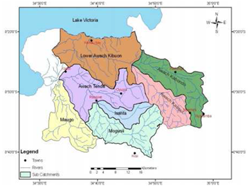
1.1. Description of the Study AreaThe area of the study is the Upper Awach-Kasipul sub-catchment (part of the larger Awach-Kibuon catchment) located in Nyamira County. The larger Awach Catchment (Figure 1) is part of the Lake Victoria South Catchment Area (LVSCA) and flows North West (NW) into Lake Victoria around the port of Kendu Bay Figure 1. The Kibuon River is 52 km long and has a catchment area is 760 km2.
According to the 2009 census the population of Nyamira County was estimated to be 598,252 and projected to be 632,046 persons in 2012. Approximately 46.3% fall below the poverty line and this is high compared to Kenya’s poverty rate which is projected to be in the range of 34 and 42 percent (Kenya Economic Update 2013; World Bank 12). The food poor are estimated to be around 21.8% and 1.9% are the hard-core poor who cannot afford poor even when they spend all their income on food.
In order to address poverty, the 14 proposes development programs such as intensive farming, improvement in electricity connectivity, maintenance of roads and establishment of cottage industries for processing agricultural produce. Only a few farmers (8%) are practicing any type of irrigation and another (15%) who have on farm experience on irrigated agriculture.
The crop choice under irrigation is based on the suitability for various crops to soils, climate, topography, both in long and short rain seasons; as well as water availability, particularly in the months of September -March; to take advantage of the rained agriculture development as much as possible.
1.2. Objectives of the StudyThe objective of this research study was to assess the available water that can be put to other uses such as irrigation water demand, domestic water requirement after due consideration to the environmental flow. The available water was estimated by deducting the following from the 80% probable flows orQ80: i) Deduction of estimated existing/future abstractions- determined from available information on irrigation activities along the three rivers (upstream and downstream) and ii) Deduction of the environmental flow - taken as 30% of the Q95 probable flow based on monthly mean flows. Q80 is the is the flow that is exceeded 80 % of the time, e.g. 4 out of 5 years. Environmental or reserve flow (Q95) is the flow that must be released to meet ecological needs downstream and normally used as a design criterion for domestic water supplies); while Q50 is the flood flow.
This section outlines the source and characteristics of data used in the analysis, and the steps involved in the analysis, which include estimation of missing data, estimation of flow discharge using both the rating formula and the curve number methods, flood frequency and probability of exceedance analyses.
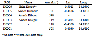
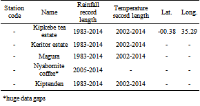
2.1. DataDaily discharge data was obtained from Water Management Authority (Kisii sub-regional office) while daily rainfall data from the Kenya Meteorological Department (KMD) Headquarters in Nairobi.. The Rated Gauging Station (RGS) 1HD06 at Eaka had only water level data available over a period of 7 years, while the rest of the RGSs had flow data. With the exception of Nyabomite coffee factory rainfall station which had less than10 years of data, the rest had more than 20 years of data. A list of flow and rainfall stations used is summarized in Table 1a and 1b.
The following sub-section involves estimation of missing data, calculation of discharge for specific return periods, estimation of flow duration curves and computation of available water for irrigation.
2.2. MethodologyThe Local Regression or Locally weighted polynomial regression (LOESS) was used to estimate missing data 15, 16. At each point in the data set a low-degree polynomial is fitted to a subset of the data, with explanatory variable values near the point whose response is being estimated. The polynomial is fitted using weighted least squares, giving more weight to points near the point whose response is being estimated and less weight to points further away. The value of the regression function for the point is then obtained by evaluating the local polynomial using the explanatory variable values for that data point. The LOESS fit is complete after regression function values have been computed for each of the data points. Many of the details of this method, such as the degree of the polynomial model and the weights, are flexible. The range of choices for each part of the method and typical defaults are briefly discussed. The weighting factor for input data point i is a sigmoidal curve based on equation 1:
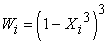 | (1) |
Where  is the normalized distance (along the X axis) between input data point i and the output X value at which the LOESS smoothed value is being computed. The normalization X is the distance/ (maximum distance among points in the moving regression).
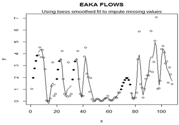
Apart from being simple, this method provides a specification of a function that fits a model to all the data in the sample, thus requiring the smoothing parameter value and not the local polynomial. Additionally, it is possible to model complex processes for which no theoretical model exists due to its simplicity. To estimate missing data for Eaka at 1HD06, this method is used. The estimates are plotted in Figure 2, with the X axis indicating years and the y-axis displaying the water levels.
As mentioned earlier, Eaka at 1HD06 had only water level data. To be able to use this station data in the analysis, the water levels had to be converted into discharge. Both the rating formula and the Curve Number (CN) methods were used to convert water levels to discharge. The rating formula was first used to obtain flow values, and the CN method used to obtain values for verification.
The rating formula was used to obtain discharge for stations with water level data only. The rating equation is expressed as in equation 2 where Q is the discharge (m3/s), α is the stage for zero discharge (meters), G is the gauge depth (meters) while Cr and β are coefficients 17.
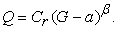 | (2) |
The equation becomes:
 | (3) |
 | (4) |
 and
and  from equations 3 and 4 can be calculated using equations 5 and 6
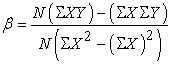 | (5) |
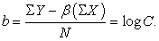 | (6) |
The coefficient of correlation can be estimated using equation 7 where a running method can be used to estimate the constant α 17:
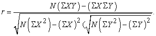 | (7) |
The constants for the station Eaka at 1HD06 are estimated as: C=16.453, α=0.216 and β=2.397, thus producing equation 8 as the final rating formula.
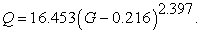 | (8) |
In hydrology, the quantification of design peak discharges on data-scarce catchments has been a continuing problem 8, 18. Precise estimates of flood quantiles are needed for efficient design of hydraulic structures 19, 20; however, historical data that are required to quantify the flood statistics are usually unavailable at the site of interest or the available information may not be representative of the catchment studied because of the changes in the watershed characteristics, such as urbanization 8, 21.
The measured hydrological data, particularly in developing countries such as Kenya can be limited, short, or nonexistent to the extent that they are far from representative of the basin under consideration 18, 22. In this paper, the Curve number method has been used to estimate run off depth from rainfall where the former was not available.
The Curve Number (CN) method or the Soil Conservation service (SCS) Curve number method was developed by the US Soil Conservation Service for agricultural purposes 23. In this approach a simple empirical formula and readily available tables and curves are used. The CN is a crucial factor to consider for runoff estimation 24. A high curve number means high runoff and low infiltration; whereas a low curve number means little runoff and high infiltration 25. The curve number is a function of land use and Hydrologic Soil Group (HSG). It is a method that can incorporate the land use for the computation of runoff from rainfall. The SCS-CN method provides a rapid way to estimate runoff change due to land use change 25.
Using this approach, the run off depth, Q from the sub-basin can be estimated using equation 9. In this equation, P represents the basin average rainfall estimated from available rainfall records and S is the potential maximum retention of the soil (in mm) after runoff begins and is related to the soil and land cover conditions of the watershed. S can be related to the CN as given in equation 10.
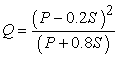 | (9) |
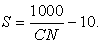 | (10) |
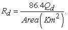
The CN can be estimated from the land cover type and the hydrologic soil group for the region (s) of interest. Soil group classifications for the USA can be referred at SCS 23 but classifications based on East African conditions are documented by Springer 26. The land cover type for the Upper Awach-Kibuon is considered to be good (grass cover >75%) with a hydrologic soil group D which provides a maximum infiltration rate. The curve number for these types of conditions is estimated to be equal to 80. Hence, from equation 10, S was estimated to be equal to 1.111. It should be noted that the runoff depths Q generated in equation 9 are equivalent to effective rainfall series  in mm given by equation 11, where Qd is the required series of discharge. The catchment area corresponding to RGS 1HD06 is 39 km2. This value was used to convert the run-off depths in equation 11 to estimate discharge in equation 9. The discharge calculated using the CN method was compared to those by the rating formula, and these values used to compute the exceedance/non-exceedance probabilities.
 | (11) |
Flood frequency analysis involves the calculation of flow values that correspond to specific return periods. The return period T (in years) of an event was given as a function of the General Extreme Value (GEV) function (equation 12).
 | (12) |
If F(x) represents the distribution of the annual maximum series, T is calculated using equations 13 and 14, where  represents the population survival function.
 | (13) |
 | (14) |
The inverse distributions for these equations can be calculated using equations 15 and 16, where x is the discharge value corresponding to specific F(x) and α, β and  the location, shape and scale parameters respectively. The values of x represent discharge at specific return periods.
 | (15) |
 | (16) |
A flow duration curve indicates the percentage of time the river discharge (either daily, monthly or annually) is exceeded over a given period. Flow duration is represented by an empirical exceedance frequency E (equation 17), where t- represents the stream flow rank (flow records sorted in descending order), and s the sample size considered.
 | (17) |
The exceedance frequency for high flows is calculated using equation 18 where XE is the exceedance level while G denotes a GEV distribution to which the flows fit into. The exceedance frequency for high flows with an exponential distribution can therefore be calculated using equation 19
 | (18) |
 | (19) |
The E-percentage event can then be calculated using equation 20 where t represents the number of observations above the threshold, s the sample size, β the location parameter and xt the threshold discharge.
 | (20) |
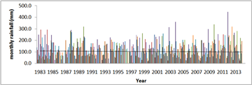
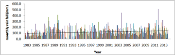
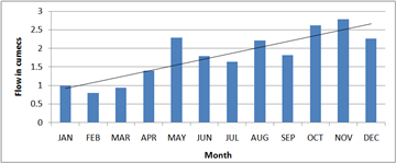
This section presents the results of the analyses and a brief discussion on their implications. An analysis of the rainfall and temperature time series shows that the monthly maximum temperature has an increasing trend while the minimum monthly temperature is on a general decrease. This implies a steady increase in the temperature ranges for this area. The hightemperature in this sub-catchment may also suggest a high rate of evaporation.. Monthly rainfall at Keritor and Magura estate rainfall stations show a slight increasing trend and decreasing trend respectively for Keritor and Magura respectively (Figure 3a and Figure 3b); and the mean monthly flows also indicate an increasing trend (Figure 3c). It is also observed that the rainfall values however have a high variability across the years. The years 2005 and 2013 have the highest monthly rainfall recorded, with values of more than 450 mm. The positive trend in monthly rainfall suggests an increase in the risk of flooding.
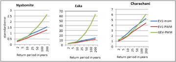
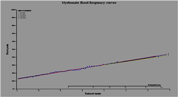
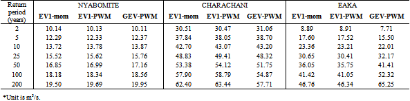
Results from the flood frequency analysis are displayed in Table 2, as estimated from the General Extreme Value and Extreme Value type 1 distribution using the methods of moments (mom), maximum likelihood (ML) and Probability Weighted Moments (PWM) to estimate the parameters of the distribution. The best distribution is the EV1-PWM since it has the lowest standard error for all the RGS (Figure 4).
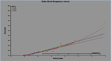
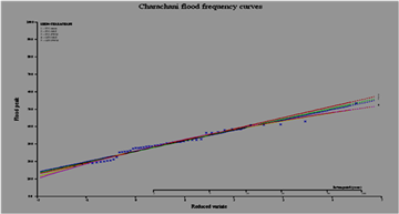
The flow discharges corresponding to specific return periods are therefore estimated using the EV1-PMW method (Figure 5). At each of the return periods, the results indicate relatively higher discharge values for Charachani compared to Eaka and Nyabomite, suggesting bigger floods at this location relative to the other locations. This further suggests a need for larger flood control structures at Charachani, as the discharges at this location are twice those at Nyabomite and Eaka.
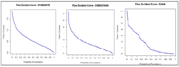
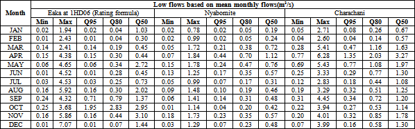
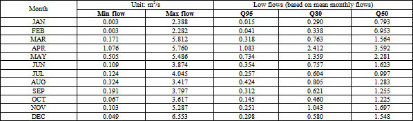
Exceedance probabilities are used to construct flow duration curves, which display the chance that a given flow is exceeded in a given time period. The exceedance probabilities at Eaka, Charachani and Nyabomite were calculated based on mean monthly flow records. Results show that high flow values have low probabilities of exceedance and vice versa. Actual flow values vary from one location to another. At all exceedance probabilities, Charachani has the highest flows as compared to the other two stations (Table 3). Table 4 shows the exceedance probabilities of flows at Eaka, calculated using discharge values estimated by the CN method. The annual flow duration curves are plotted in Figure 6.
The probabilities of exceedance were used to estimate the water available for irrigation at the different gauging stations in the sub-catchment. The available flow for irrigation and the environmental flow are crucial in this process. The available flow for irrigation is calculated from Q80 (also called the natural flow, i.e. flow exceeded 4 out of 5 times in a year) and the environmental flow computed from Q95 i.e. flow exceeded 95% of the times. Environmental concerns are foremost on the minds of administrators, planners, and the general populace, with the result that there is a steadily increasing awareness and emphasis on the requirements of environmental flows in any river system toward maintaining ecosystems such as wetland and in-stream environs 27. Computed values of Q80, Q90 and Q95 are shown in Table 3. The difference between the environmental and natural flow gives estimates of the available water for irrigation purposes. Kenyan regulations require that 30% of the Q95 base flow be considered as the environmental flow. The available water for irrigation is therefore calculated from equation 21. This formula is also called the water balance calculation for irrigation water requirement. Results for the available water at each RGS are shown in Table 5.
Give the actual figures or values
 | (21) |
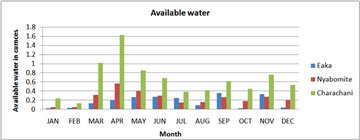
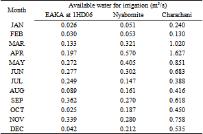
Note: The available water is calculated on a monthly basis for each of the three locations. Figure 7 and Table 5 below indicate the amount of water that can be extracted in this case for irrigation purposes after satisfying the environmental flow.
From the results, a larger volume of water is available for irrigation at Charachani, for example, lowest being 0.388 cumecs in the month of July compared to 0.147 cumecs for Nyabomite and 0.249 cumecs for Eaka. The largest amount of water for irrigation is available during the months of May and November, with peaks corresponding to those of the rainy seasons. The months with the least available water for irrigation are December, January and February, which also corresponds with the dry seasons.
The management of water resources most often may require the quantification and determination of the frequency and magnitude of flow events that will occur at the water management areas or units. The frequency analysis define the relationship between the magnitude and the frequency of an event, for which that event is exceeded.. The probabilities of exceedance, for example, can be used to estimate the water available for irrigation purposes. This is especially relevant to a region like the Awach-Kibuon sub-catchment, which even though makes a considerable contribution to the country’s food security due to its high agricultural potential; it is still faced with threats arising from frequent droughts which often threatens rainfed agriculture.. This paper sought to carry out a hydrological assessment that can inform the design, construction of flow control structures and estimation of available water that could be extracted from nearby water resources (Eaka-Nyabomite-Charachani streams) for irrigation purposes. The available water was estimated by deducting the following from the 80% probable flows or Q80: i) Deduction of estimated existing/future abstractions- determined from available information on irrigation activities along the three rivers (upstream and downstream) and ii) Deduction of the environmental flow - taken as 30% of the Q95 probable flow based on monthly mean flows
From the results, a larger volume of water is available for irrigation at Charachani, for example,lowest being 0.388 cumecs in the month of July compared to 0.147 cumecs for Nyabomite and 0.249 cumecs for Eaka.. The largest amount of water for irrigation is available during the months of May and November, with peaks corresponding to those of the rainy seasons. The months with the least available water for irrigation are December, January and February, which also corresponds with the dry seasons. Refining these results to take into account the present and future challenges will require use of gridded data sources such as NOAA, NCEP, CPC to augment the scarce observations. Moreover, climate projections may be useful in order to keep pace with the challenges of climate change.
The author is grateful to the financial support from the National Irrigation Board (NIB), Kenya through Quadrant Engineering Consultants. The latter was the consulting firm for the Feasibility Study, Detailed Design and Preparation of Tender Documents for Nyabomite Cluster Irrigation Development Project, Nyamira County.
| [1] | Ahmad, U.N., Shabri, A., and Zakaria, Z.A., (2011): Flood frequency analysis of annual maximum stream flows using L-Moments and TL-Moments. Applied Mathematical Sciences, vol. 5, pp. 243- 253. | ||
| In article | |||
| [2] | Noto, L., and G. La Loggia. 2009. “Use of L-Moments Approach for Regional Flood Frequency Analysis in Sicily, Italy.” Water Resources Management 23 (11): 2207-29. | ||
| In article | View Article | ||
| [3] | Balica, S. F., I. Popescu, L. Beevers, and N. G. Wright. 2013. “Parametric and Physically Based Modelling Techniques for Flood Risk and Vulnerability Assessment: A Comparison.” Environmental Modelling & Software 41: 84-92. | ||
| In article | View Article | ||
| [4] | Cunnane, C. 1989. “Statistical Distributions for Flood Frequency Analysis.” In Operational Hydrology Report | ||
| In article | |||
| [5] | England, J. F., Jr., T. A. Cohn, B. A. Faber, J. R. Stedinger, W. O. Thomas, Jr., A. G. Veilleux, J. E. Kiang, and R. R. Mason, Jr. 2018. “Guidelines for determining flood flow frequency—Bulletin 17C.” Chap. B5 in USGS Techniques and Methods, Book 4. Reston, VA: USGS. | ||
| In article | View Article | ||
| [6] | Oosterbaan, R.J. Frequency and Regression Analysis of Hydrologic Data. Part I: Frequency Analysis. Drainage Principles and Applications, Publication 16. Chapter 6; Ritzema, H.P., Ed.; International Institute for Land Reclamation and Improvement (ILRI):Wageningen, The Netherlands, 1994. | ||
| In article | |||
| [7] | Hosking, J.R.M.; Wallis, J.R. Regional Frequency Analysis: An Approach Based on L-moments; Cambridge University Press: Cambridge, UK, 2005. | ||
| In article | |||
| [8] | Hailegeorgis, T.T.; Alfredsen, K. Regional flood frequency analysis and prediction in ungauged basins including estimation of major uncertainties for mid-Norway. J. Hydrol. Reg. Stud. 2017, 9, 104-126. | ||
| In article | View Article | ||
| [9] | Chen, X.; Shao, Q.; Xu, C.-Y.; Zhang, J.; Zhang, L.; Ye, C. Comparative study on the selection criteria for fitting flood frequency distribution models with emphasis on upper-tail behavior. Water 2017, 9, 320. | ||
| In article | View Article | ||
| [10] | Rizwan, M.; Guo, S.; Xiong, F.; Yin, J. Evaluation of various probability distributions for deriving design flood featuring right-tail events in pakistan. Water 2018, 10, 1603. | ||
| In article | View Article | ||
| [11] | Bezak, N.; Brilly, M.; Šraj, M. Comparison between the peaks-over-threshold method and the annualmaximum method for flood frequency analysis. Hydrol. Sci. J. 2014, 59, 959-977. | ||
| In article | View Article | ||
| [12] | World Bank (2013): Kenya Economic update June, 2013. Edition No.8 | ||
| In article | |||
| [13] | The Study on the National Water Master Plan, Ministry of Water Development, 2014. | ||
| In article | |||
| [14] | County Integrated Development Plan (CIDP) 2013-2018 for Nyamira County, Kenya. | ||
| In article | |||
| [15] | Cleveland, W.: Robust Locally Weighted Regression and Smoothing Scatterplots. Jour. of the American Statistical Association, 74(368), p.829, 1979 | ||
| In article | View Article | ||
| [16] | Cleveland, W. and Devlin, S.: Locally Weighted Regression: An Approach to Regression Analysis by Local Fitting. Jour. of the American Statistical Association, 83(403), pp.596-610, 1988. | ||
| In article | View Article | ||
| [17] | Subramanya, K.: Flow in open channels, Tata McGraw-Hill publishing Co., New Delhi, 2007. | ||
| In article | |||
| [18] | Tegegne, G.; Kim, Y.-O. Modelling ungauged catchments using the catchment runo_response similarity. J. Hydrol. 2018, 564, 452-466. | ||
| In article | View Article | ||
| [19] | Tegegne, G.; Kim, Y.-O. Strategies to enhance the reliability of flow quantile prediction in the gauged and ungauged basins. River Res. Appl. 2020, 36, 724-734. | ||
| In article | View Article | ||
| [20] | Tegegne, G.; Kim, Y.-O.; Seo, S.B.; Kim, Y. Hydrological modelling uncertainty analysis for di_erent flow quantiles: A case study in two hydro-geographically different watersheds. Hydrol. Sci. J. 2019, 64, 473-489. | ||
| In article | View Article | ||
| [21] | Ouarda, T.; Cunderlik, J.M.; St-Hilaire, A.; Barbet, M.; Bruneau, P.; Bobée, B. Data-based comparison of seasonality-based regional flood frequency methods. J. Hydrol. 2006, 330, 329-339. | ||
| In article | View Article | ||
| [22] | Tegegne, G.; Park, D.K.; Kim, Y.-O. Comparison of hydrological models for the assessment of water resources in a data-scarce region, the Upper Blue Nile River Basin. Journal of Hydrology: Regional Studies (2017) 14 49-66. | ||
| In article | View Article | ||
| [23] | Soil Conservation Service: National engineering handbook, Section 4, Hydrology. Department of Agriculture, Washington, 762pp, 1972. | ||
| In article | |||
| [24] | Bonta J. V. (1997). Determination of watershed curve number using derived distributions. Journal of Irrigation and Drainage Engineering, 123(1), 28-36. | ||
| In article | View Article | ||
| [25] | Xiaoyong Zhan, Min-Lang Huang (2004). ArcCN-Runoff: an ArcGIS tool for generating curve number and runoff maps, Environmental Modelling & Software, 27-04-04 13:11:52 3B2 Ver.: 7.51c/W Model: 5 ENSO1500. | ||
| In article | |||
| [26] | Sprenger, F.D.: Determination of direct runoff with the 'Curve Number Method' in the coastal area of Tanzania/East Africa. Wasser und Boden, I, pp. 13-16, 1978. | ||
| In article | |||
| [27] | Opere A. (2020): Integrated Water Management to Meet Competing Demands in Agricultural and Other Sectors. In: Leal Filho W., Azul A., Brandli L., Özuyar P., Wall T. (eds) Zero Hunger. Encyclopedia of the UN Sustainable Development Goals. Springer, Cham | ||
| In article | View Article | ||
Published with license by Science and Education Publishing, Copyright © 2020 Opere A.O. and A.K. Njogu
![]() This work is licensed under a Creative Commons Attribution 4.0 International License. To view a copy of this license, visit
http://creativecommons.org/licenses/by/4.0/
This work is licensed under a Creative Commons Attribution 4.0 International License. To view a copy of this license, visit
http://creativecommons.org/licenses/by/4.0/
| [1] | Ahmad, U.N., Shabri, A., and Zakaria, Z.A., (2011): Flood frequency analysis of annual maximum stream flows using L-Moments and TL-Moments. Applied Mathematical Sciences, vol. 5, pp. 243- 253. | ||
| In article | |||
| [2] | Noto, L., and G. La Loggia. 2009. “Use of L-Moments Approach for Regional Flood Frequency Analysis in Sicily, Italy.” Water Resources Management 23 (11): 2207-29. | ||
| In article | View Article | ||
| [3] | Balica, S. F., I. Popescu, L. Beevers, and N. G. Wright. 2013. “Parametric and Physically Based Modelling Techniques for Flood Risk and Vulnerability Assessment: A Comparison.” Environmental Modelling & Software 41: 84-92. | ||
| In article | View Article | ||
| [4] | Cunnane, C. 1989. “Statistical Distributions for Flood Frequency Analysis.” In Operational Hydrology Report | ||
| In article | |||
| [5] | England, J. F., Jr., T. A. Cohn, B. A. Faber, J. R. Stedinger, W. O. Thomas, Jr., A. G. Veilleux, J. E. Kiang, and R. R. Mason, Jr. 2018. “Guidelines for determining flood flow frequency—Bulletin 17C.” Chap. B5 in USGS Techniques and Methods, Book 4. Reston, VA: USGS. | ||
| In article | View Article | ||
| [6] | Oosterbaan, R.J. Frequency and Regression Analysis of Hydrologic Data. Part I: Frequency Analysis. Drainage Principles and Applications, Publication 16. Chapter 6; Ritzema, H.P., Ed.; International Institute for Land Reclamation and Improvement (ILRI):Wageningen, The Netherlands, 1994. | ||
| In article | |||
| [7] | Hosking, J.R.M.; Wallis, J.R. Regional Frequency Analysis: An Approach Based on L-moments; Cambridge University Press: Cambridge, UK, 2005. | ||
| In article | |||
| [8] | Hailegeorgis, T.T.; Alfredsen, K. Regional flood frequency analysis and prediction in ungauged basins including estimation of major uncertainties for mid-Norway. J. Hydrol. Reg. Stud. 2017, 9, 104-126. | ||
| In article | View Article | ||
| [9] | Chen, X.; Shao, Q.; Xu, C.-Y.; Zhang, J.; Zhang, L.; Ye, C. Comparative study on the selection criteria for fitting flood frequency distribution models with emphasis on upper-tail behavior. Water 2017, 9, 320. | ||
| In article | View Article | ||
| [10] | Rizwan, M.; Guo, S.; Xiong, F.; Yin, J. Evaluation of various probability distributions for deriving design flood featuring right-tail events in pakistan. Water 2018, 10, 1603. | ||
| In article | View Article | ||
| [11] | Bezak, N.; Brilly, M.; Šraj, M. Comparison between the peaks-over-threshold method and the annualmaximum method for flood frequency analysis. Hydrol. Sci. J. 2014, 59, 959-977. | ||
| In article | View Article | ||
| [12] | World Bank (2013): Kenya Economic update June, 2013. Edition No.8 | ||
| In article | |||
| [13] | The Study on the National Water Master Plan, Ministry of Water Development, 2014. | ||
| In article | |||
| [14] | County Integrated Development Plan (CIDP) 2013-2018 for Nyamira County, Kenya. | ||
| In article | |||
| [15] | Cleveland, W.: Robust Locally Weighted Regression and Smoothing Scatterplots. Jour. of the American Statistical Association, 74(368), p.829, 1979 | ||
| In article | View Article | ||
| [16] | Cleveland, W. and Devlin, S.: Locally Weighted Regression: An Approach to Regression Analysis by Local Fitting. Jour. of the American Statistical Association, 83(403), pp.596-610, 1988. | ||
| In article | View Article | ||
| [17] | Subramanya, K.: Flow in open channels, Tata McGraw-Hill publishing Co., New Delhi, 2007. | ||
| In article | |||
| [18] | Tegegne, G.; Kim, Y.-O. Modelling ungauged catchments using the catchment runo_response similarity. J. Hydrol. 2018, 564, 452-466. | ||
| In article | View Article | ||
| [19] | Tegegne, G.; Kim, Y.-O. Strategies to enhance the reliability of flow quantile prediction in the gauged and ungauged basins. River Res. Appl. 2020, 36, 724-734. | ||
| In article | View Article | ||
| [20] | Tegegne, G.; Kim, Y.-O.; Seo, S.B.; Kim, Y. Hydrological modelling uncertainty analysis for di_erent flow quantiles: A case study in two hydro-geographically different watersheds. Hydrol. Sci. J. 2019, 64, 473-489. | ||
| In article | View Article | ||
| [21] | Ouarda, T.; Cunderlik, J.M.; St-Hilaire, A.; Barbet, M.; Bruneau, P.; Bobée, B. Data-based comparison of seasonality-based regional flood frequency methods. J. Hydrol. 2006, 330, 329-339. | ||
| In article | View Article | ||
| [22] | Tegegne, G.; Park, D.K.; Kim, Y.-O. Comparison of hydrological models for the assessment of water resources in a data-scarce region, the Upper Blue Nile River Basin. Journal of Hydrology: Regional Studies (2017) 14 49-66. | ||
| In article | View Article | ||
| [23] | Soil Conservation Service: National engineering handbook, Section 4, Hydrology. Department of Agriculture, Washington, 762pp, 1972. | ||
| In article | |||
| [24] | Bonta J. V. (1997). Determination of watershed curve number using derived distributions. Journal of Irrigation and Drainage Engineering, 123(1), 28-36. | ||
| In article | View Article | ||
| [25] | Xiaoyong Zhan, Min-Lang Huang (2004). ArcCN-Runoff: an ArcGIS tool for generating curve number and runoff maps, Environmental Modelling & Software, 27-04-04 13:11:52 3B2 Ver.: 7.51c/W Model: 5 ENSO1500. | ||
| In article | |||
| [26] | Sprenger, F.D.: Determination of direct runoff with the 'Curve Number Method' in the coastal area of Tanzania/East Africa. Wasser und Boden, I, pp. 13-16, 1978. | ||
| In article | |||
| [27] | Opere A. (2020): Integrated Water Management to Meet Competing Demands in Agricultural and Other Sectors. In: Leal Filho W., Azul A., Brandli L., Özuyar P., Wall T. (eds) Zero Hunger. Encyclopedia of the UN Sustainable Development Goals. Springer, Cham | ||
| In article | View Article | ||


