1. Introduction

Fractional order partial differential equations are generalizations of classical partial differential equations ^{[1, 2, 3, 4]}. It has been of considerable interest in the recent literature. This topic has received a great deal of attention especially in the fields of viscoelasticity materials, electrochemical processes, dielectric polarization, colored noise, anomalous diffusion, signal processing, control theory and others. Increasingly, these models are used in applications such as fluid flow, finance and others. A Fokker–Planck equation (FPE) has commonly been used to describe the Brownian motion of particles ^{[18, 19, 20, 21]}. An FPE describes the change of probability of a random function in space and time; hence it is naturally used to describe solute transport. The general FPE for the motion of a concentration field U(x,t) of one space variable x at time t has the form ^[18]. The Fractional Fokker–Planck equation has recently been treated by a number of authors. Liu et al. ^{[22, 23]} presented practical numerical methods to solve the space Fractional Fokker–Planck equation. Metzler et al. ^[24] obtained a solution for the Fractional Fokker–Planck equation (4) using separation of variables. However, the analytic solution of most Fractional Fokker–Planck equation cannot be obtained explicitly.

Most nonlinear fractional differential equation do not have analytic solutions, so approximation and numerical techniques must be used. The Adomian decomposition method and the variational iteration method ^{[5, 6, 7, 8, 9]} are relatively new approaches to provide analytical approximation to linear and nonlinear problems ^[10]. The structure of this paper is as follows. We begin by introducing some basic definitions and mathematical preliminaries of the fractional calculus theory which are required for establishing our results. In section 2, we get the general from numerical solution to Fokker – Planck equation with time- fractional derivatives by used the Adomian Decomposition Method. In section 3, also we solve the fractional linear Fokker – Planck equation by using the variational iteration method. (We extend the application of the Adomian decomposition method to construct our numerical solutions for the fractional linear Fokker – Planck equation). In section 4, we present two examples to show the efficiency and simplicity of the methods.

Definition: The fractional derivative ofin the Caputo sense is defined as

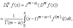(1)

For .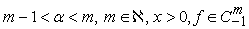

Caputo’s definition n which is a modification of the Riemann- Liouville definition and has the advantage of dealing properly with initial value problems in which the initial conditions are given in term's of the field variable and their integer order which is the case in most physical processes.

Properties of the operator can be found in ^{[1, 3, 4]}, we mention only the following:

For 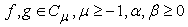and

.

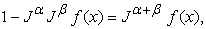
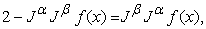
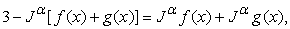
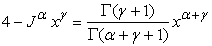Also we need here two of its basic properties.

Lemma: if 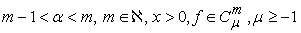, then

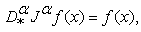(2)

and

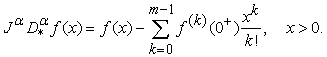(3)

2. Adomian Decomposition Method (ADM)

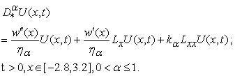
In this section we solve the time-fractional Fokker-Planck equation by the Adomian's decomposition method; we consider the time-fractional Fokker-Planck equation.

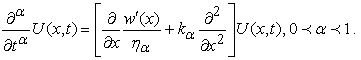(4)

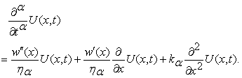(5)

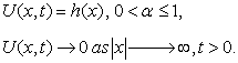
With the initial condition

(6)

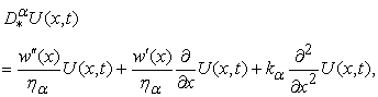
The standard form of the time-fractional Fokker-Planck equation in an operator from is

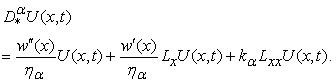(7)

Where is the Caputo fractional derivative of order, is defined as in Eq.(3), and .

The method is based on applying the operator, the inverse of the operator, on both sides of Eq. (7) to obtain

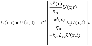(8)

The Adomian's decomposition method [5-12]^[5] assumes a series solution for is given by

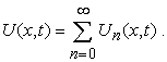(9)

Substituting the decomposition series (9) into (8) gives

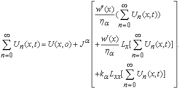(10)

From this equation, the iterates are defined by the following recursive way

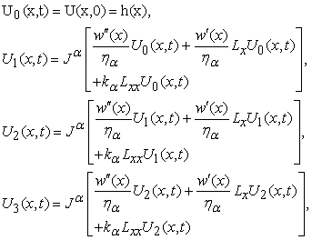(11)

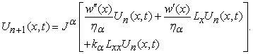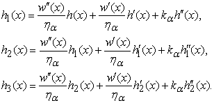
Using the above recursive relationship, the first few terms of the decomposition series are given

(12)

Hence

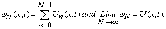
The solution in series form is given by

(13)

Where

(14)

Finally, we approximate the solution by truncated series

3. Variationalal Iteration Method (VIM)

In this section we solve the time-fractional Fokker-Planck equation by the variationalal iteration method ^{[13, 14, 15, 16]}, We consider the time-fractional Fokker-Plnack equation

(15)

Where is the Caputo fractional derivative of order, is defined as in Eq.(1).

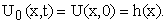
The initial condition associated with (15) is of the form

(16)

The correction function for Eq.(15) can be approximately expressed as follows:

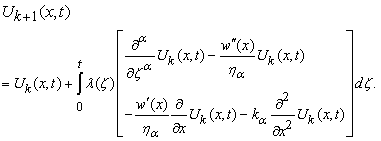(17)

Where is a general Lagrange multiplier ^[17].

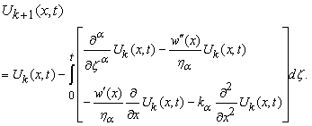
For 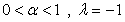then the correction functional become

(18)

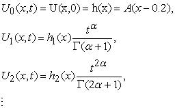
In this case we begin with the initial approximation

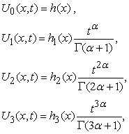
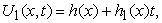
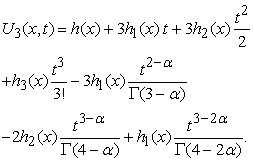
By the above variationalal iteration formula (18), we can obtain the following approximations:

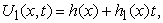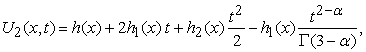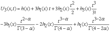(19)

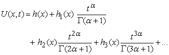
Where and are defined by Eq.(14). Therefore the solution in series form is given by

then

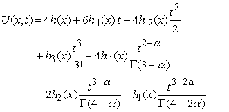(20)

and the exact solution is obtained as

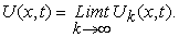4. Numerical Experiments

In this section we shall illustrate

Example 4-1: Consider classical Fokker-Planck equation[]

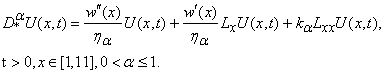(21)

Subject to the initial condition

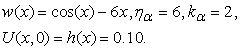(22)

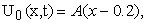
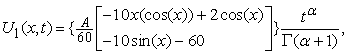
First Adomian Decomposition Method

To solve the problem by using the Adomian decomposition method, from Eq.(13), which represent the first few terms of the decomposition series

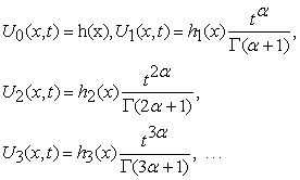(23)

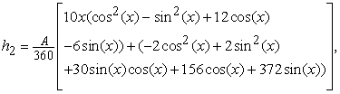
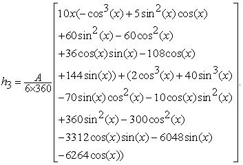
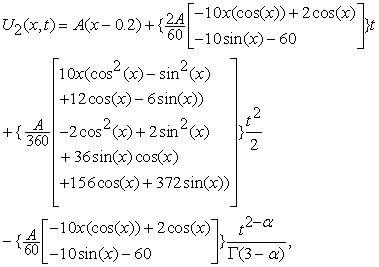
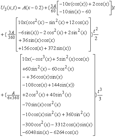
then, the first terms of the decomposition series are

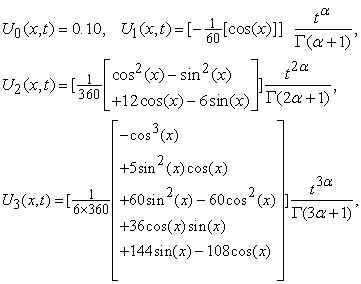(24)

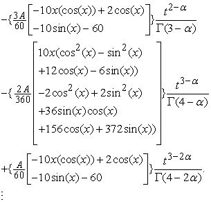
and so on, in the same manner the rest of the components of the decomposition series can be obtained

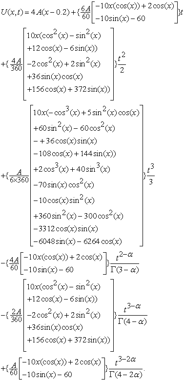
Hence

The solution in series form is given by

(25)

In the following we introduce the behavior of the numerical solution of the Fokker-Planck equation using the Adomian Decomposition Method.

Figure 1. The evolution of u(x,t) with absorbing boundary conditions, where the dotted line “stands for the solution when t=0.3”, the dot dashed line “stands for the solution when t=0.6”, the dashed line “stands for the solution when t=1”

Download as

PowerPoint Slide

Larger image(png format)

Figures index

Veiw figure

View current figure in a new window

View next figure

Second Variationalal Iteration Method

We solve the problem by using variationalal iteration method, according to Eq.(19), The first few terms of the decomposition series are given:

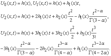(26)

From Eq.(13), Eq.(22), Eq.(24) and Eq.(26), then

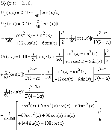(27)

Hence

The solution in series form is given by

(28)

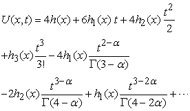Then the exact solution can be expressed as follows:

(29)

Figure 2. The evolution of u(x,t) with absorbing boundary conditions, where the dotted line “stands for the solution when t=0.3”, the dot dashed line “stands for the solution when t=0.6”, the dashed line “stands for the solution when t=1”

Download as

PowerPoint Slide

Larger image(png format)

Figures index

Veiw figure

View current figure in a new window

View previous figure

View next figure

In the following we introduce the behavior of the numerical solution of the Fokker-Planck equation using the Varitional Iteration Method.

Some numerical results

Numerical Results For Example 1:

Table 1. The numerical solution of the Fokker-Planck equation using the Adomian Decoposition and Variationalal Iteration Methods for different values of α for t=0.3, 0.6 and 1

Download as

PowerPoint Slide

Larger image(png format)

Tables index

Veiw figure

View current table in a new window

View next table

Example 4-2: Consider classical Fokker-Planck equation

(29)

Subject to the initial condition

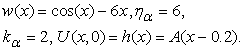(30)

Where is constant.

First Adomian Decomposition Method

To solve the problem using the Adomian Decomposition Method, then the first few terms of the decomposition series are,

(31)

From Eq.(14) and Eq.(31), then we get

(32)

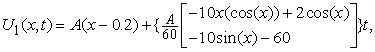
Then, the first terms of the decomposition series becomes

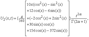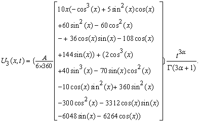(33)

and so on, in the same manner the rest of the components of the decomposition series can be obtained.

Hence

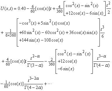
The solution in series form is given by

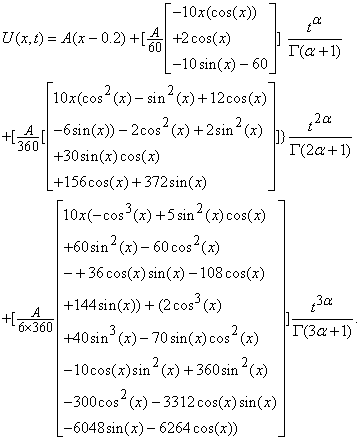(34)

Figure 3. The evolution of u(x,t) with absorbing boundary conditions, where the dotted line “stands for the solution when t=0.3”, the dot dashed line “stands for the solution when t=0.6”, the dashed line “stands for the solution when t=1”, when A=0.5

Download as

PowerPoint Slide

Larger image(png format)

Figures index

Veiw figure

View current figure in a new window

View previous figure

View next figure

Second Variationalal Iteration Method

We solve the problem by using Variationalal Iteration Method, according to Eq.(19), the first few terms of the decomposition series are given:

(35)

From Eq.(33) and Eq.(31), then the first few terms of the decomposition series becomes

(36)

and so on, in the same manner the rest of the components of the iteration formula (18) can be obtained using the Mathematic package.

Hence

The solution in series form is given by

(37)

Figure 4. The evolution of u(x,t) with absorbing boundary conditions, where the dotted line “stands for the solution when t=0.3”, the dot dashed line “stands for the solution when t=0.6”, the dashed line “stands for the solution when t=1”, when A=0.5.

Download as

PowerPoint Slide

Larger image(png format)

Figures index

Veiw figure

View current figure in a new window

View previous figure

Some numerical results:

Table 2. The numerical solution of the Fokker-Planck equation using the Adomian Decoposition and Variationalal Iteration Methods for different values of α for t=0.3, 0.6 and 1 when A=0.5

Download as

PowerPoint Slide

Larger image(png format)

Tables index

Veiw figure

View current table in a new window

View previous table

5. Conclusion

The fundamental goal of this paper was to construct an approximate solution of fractional Fokker-Plank equation. The goal is achieved by using the variational iteration method and the Adomian decomposition method.

The methods were used in a direct way without using linearization, perturbation or restrictive assumptions.

There are some important points to make here:

First, the variational iteration method and the decomposition method provide the solutions in terms of convergent series with easily computable components.

Second, it seems that the approximate solution of time-fractional Fokker-Plank equation using the Adomian decomposition method converges faster than the approximate solution using the variational iteration method to exact solution.

Third, Adomain decomposition method provides the components of the exact solution.

References

[1]	I.Podlubny, Fractional Differential Equations, Academic press, San Diego, (1999).
	In article
[2]	G.Samko, A.A.Kibas, O.I.Marichev, Fractional Integrals and Derivatives: Theory and Applactions, Gordon and Breach, Yverdon, (1993).
	In article
[3]	K.B.Oldham, J.Spanier, The Fractional Calculus, Academic Press, NewYork, (1974).
	In article
[4]	Y.Luchko, R.Gorenflo, The Initial Value Problem for Some Fractional Equations With Caputo Derivative, Preprint Series A08-98, Frachbreich Mathematic In Formatik, Freicumiver Siat Berlin, (1998).
	In article
[5]	G.Adpmian, Nonlinear Stochastic Systems Theory and Applications to Physics, Kluwer Academic Publishers, Dordrecht, (1989).
	In article		CrossRef
[6]	Mehdi Dehghan, Mehdi Tatari, The Use of Adomian Decomposition Method for Solving Problems in Calculus of Variational, Mathematical Problems in Engineering, (2006).
	In article		CrossRef
[7]	Sennur Somali, Guzin Gokmen, Adomian Decomposition Method For Nonlinear Strum-Liouville Problems, 2, pp 11-20, (2007).
	In article
[8]	Zaid Odibat, Shaher Momani, Numerical Methods for Nonlinear Partial Differential Equation of Fractional Order, Applied Mathematical Modeling, 32, pp 28-39, (2008).
	In article		CrossRef
[9]	A.Wazwaz, A new Algorithm for Calculation Adomian Polynomials For Nonlinear Operators, Appl. Math. Comput., 111, pp 53-69, (2000).
	In article		CrossRef
[10]	A.Wazwaz, SEl-Sayed, A new Modification of the Adomian Decomposition Method for Linear and Nonlinear Operators, Appl. Math. Comput., 122, pp 393-405, (2001).
	In article		CrossRef
[11]	Shahe Momani, An Explicit and Numerical Solution of the Fractional KDV Equation, Mathematics and Computers in Simulation, 70, pp 110-118, (2005).
	In article		CrossRef
[12]	Yong Chen, Hong-Li An, Numerical Solutions of Coupled Burgers Equations with Time-and Space-Fractional Derivatives, Appl. Math. Comput., 200, pp 87-95, (2008).
	In article		CrossRef
[13]	Zaid Odiba, Shaher Momani, Application of Variationalal Iteration Method to Nonlinear Differential Equation of Fractional Orders, Int. J. Nonlinear Sciences and Numerical Simulations, 1(7), pp 15-27, (2006).
	In article
[14]	J.H.He, Variationalal Iteration Method for Autonomous Ordinary Differential Systems, Journal Applied Mathematics and Computation Volume 114 Issue 2-3, pp 115-123, (2000).
	In article		CrossRef
[15]	J.H.He, Variationalal Principle for Nano Thin Film Lubrication, Int. J. Nonlinear Sci. Numer Simul., 4, (3), pp 313-314, (2003).
	In article		CrossRef
[16]	J.H.He, Variationalal Principle For Some Nonlinear Partial Differential Equations with Variable Coefficients, Chaos, Solitons Fractals 19 (4), pp 847-851, (2004).
	In article		CrossRef
[17]	M. Inokuti, H. Sekine,T. Mura, General use of the Lagrange multiplier in nonlinear mathematical physics, in: S. Nemat- Nasser (Ed.),Variationalal Method in the Mechanics of Solids, Pergamon Press, Oxford, pp. 156–162, (1978).
	In article
[18]	H. Risken, The Fokker–Planck Equation Springer, Berlin (1988).
	In article
[19]	Seakweng Vong, Zhibo Wang, A high order compact finite difference scheme for time fractional Fokker–Planck equations, Applied Mathematics Letters, 43, PP 38-43, (2015).
	In article
[20]	Yuxin Zhang, [3, 3] Padé approximation method for solving space fractional Fokker–Planck equations, Applied Mathematics Letters, 35, PP 109-114, (2014).
	In article
[21]	Chunhong Wu, Linzhang Lu, Implicit numerical approximation scheme for the fractional Fokker–Planck equation, Applied Mathematics and Computation, 216 ( 7), PP 1945-1955, 2010.
	In article
[22]	F. Liu, V. Anh, I. Turner, Numerical solution of space fractional Fokker–Planck equation, J. Comput. Appl. Math. Volume 166, PP 209-219, (2004).
	In article
[23]	F. Liu, V. Anh, I. Turner, Numerical simulation for solute transport in fractal porous media, ANZIAM J. (E) 45, PP 461-473. (2004).
	In article
[24]	R. Metzler, E. Barkai, J. Klafter, Anomalous diffusion and relaxation close to thermal equilibrium: a fractional Fokker–Planck equation approach, Phys. Rev. Lett. 82, PP 3563-3567, (1999).
	In article