1. Introduction

It is well known that at high data rates (typically >10 Gbit/s) polarization effects can severely impair optical communication system performance. Conventional polarization effects include polarization mode dispersion (PMD), which causes the differential group delay (DGD) between the principle states of polarization (PSPs), and polarization dependent loss (PDL), which causes polarization dependent attenuation of the propagating signal ^{[1, 2]}. DGD is a time delay at a discrete frequency between the fastest and slowest modes of an optical signal. This randomly varying delay causes optical pulses to broaden and hence bit errors. PMD is the mean of DGD over all frequencies ^[3]. State of polarization (SOP) change is caused by change of PMD and PDL ^[4]. PMD is caused by birefringence on a fiber’s core/cladding breaking the cylindrical symmetry ^[5]. The PMD describes the polarization dependence of the time delay of an optical pulse as it propagates along the fiber. High amounts of DGD can cause pulses to overlap in an optical communication system ^[6].

The PDL on a linear scale is defined as the ratio between the maximum and minimum attenuation coefficient over all polarization states. While this quantity can be measured by using scrambling and recording the maximum and minimum attenuation it is usually measured using the Jones matrix or Muller matrix method ^{[7, 8]}. PDL describes the polarization dependence of the optical attenuation for different states of polarization and can occur concurrently with PMD in fibers ^{[9, 10]}.PDL is a varying insertion loss arising from the dependence of a component’s transmission coefficient on the SOP ^[8]. In a complex system with; optical fibers, couplers, filters, multiplexers/ de-multiplexers, variable optical attenuators, erbium doped optical amplifiers, and add/drop multiplexing switchers, the combination of PMD and PDL will lead to a complex PSP vector ^{[10, 11]}.The combined PMD-PDL interaction can further degrade the system performance. Due to the interference between the fast and slow modes, the interaction between these effects will make an optical system more complicated than PMD or PDL alone. It may result in anomalous dispersion and causes additional signal distortion ^[12]. It is known that this interaction causes the fast and slow PSPs directions to become non-orthogonal ^[13]. This non-orthogonality is related to the imaginary part of the PSP vector or differential slope attenuation (DSA) ^[14].

In this paper, a new recursive formula is presented to determine the total PMD vector as a function of the local random vectors to the concatenation sections. Also, we are illustrated many treatments that may be used to study the related behavior of the random quantities in single mode fiber.

2. Statement of the Problem

Linear transmission of light from the input to the output of an optical link can always be expressed in the form

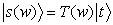(1)

where is the light frequency, and are the input and output polarization Jones vectors and is the transmission matrix. Unlike the familiar case accounting only PMD, where the transmission matrix is unitary, here is a general matrix with no significant limitations. In principal, an optical system with polarization effects can be modeled as a concatenation of segments. Each segment have the PDL and PMD effects that describe by and , respectively, which are defined as ^[3].

(2)

(3)

where is a Hermitian matrix, i.e. , which have the real eigenvalues . Note that, in this representation PDL matrix, the polarization component of field that is parallel experiences no change, but the anti-parallel component is attenuated by . The vector , which is pointing in the direction of the least attenuated state of polarization and is called PDL vector, stands for the jth PDL segment with value expressed in dB by ^[10].

(4)

The matrix is unitary, i.e. . The vector represents the local PMD vector and is the vector of Pauli spin matrices whose three components are ^[9].

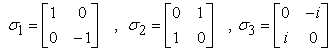(5)

Note that, for any three-dimensional vector , the product is a complex matrix.

The frequency domain evolution of the state vector may be determined by differentiating of Equation.(1) and using the fact to yield.

(6)

That may be written as

(7)

for some complex vector , where stands for PMD and is the PDL vector.

Using the definitions , where are the PSPs vectors, and , one may be found.

(8)

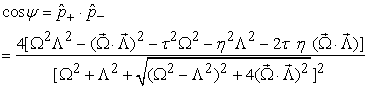
which represents the angle between the PSPs vectors in Stokes space. That is; the PSPs may be not orthogonal. More details are presented in appendix A.

3. Theoretical Representation

According to Gisin and Huttner (see Equation.(11) in Ref. ^[1]), that will make for . This means that the PDL effects are not contained in the result. In this model, we are adopted the form that makes for .

For single section, depending on the result , using Equation.(7) and the fact , yields.

(9)

Using the identities ^[5].

(10a)

(10b)

(10c)

rearrangement the result, and separating the real and imaginary parts, one may be obtained.

(11)

(12)

Using Eqs.(11) and (12), the magnitudes of and will be.

(13)

(14)

where is the angle between the local vectors and . More illustrations are explained in appendix B.

For concatenation segments, takes the form

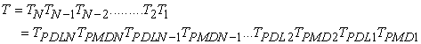(15)

Substituting Eqs.(15) and (C.1) to (C.3) into (7), see appendix C, yields

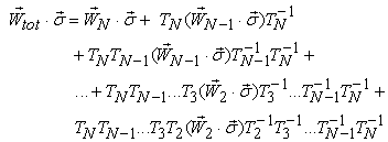(16)

where for each isolated section, we have .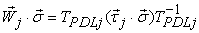

Moreover, Equation.(16) may be simplified further using the assumption 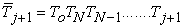to get.

(17)

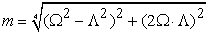
Each term in the last equation represents for one or more sections. Therefore, each term represents a traceless matrix, which can be written as . Here computed as.

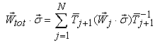
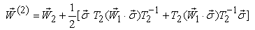
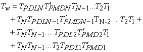
As such, the total PMD vector may be expressed as.

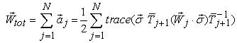(18)

Also, Equation.(18) may be reformed to obtain the following recursive relation.

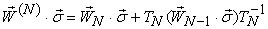(19)

where is the PMD vector of the total N segments, whereas is the PMD vector of the N-th segment only. As an example to determine , it is clear that:

and so on, where the identities in Eqs.(10) will be used to extract from . It is important to note that, the diagonal elements in the terms

are identical. Eqs.(18) and (19) represent new recursive formulas of the complex PMD vector, which give the idea about the amount of difficulties to obtain a closed form of output PMD vector that affects the propagated pulse through an optical fiber.

4. Results and Discussion

We use Equation.(18) that was derived in the above in order to simulate the phenomena PMD and PDL in single mode fiber and to extract the statistical distributions that explain the probability density function (pdf) of the parameters , , and . The selected fiber has , which is divided into concatenation sections. At each section, the local random vectors and will be generated. In turn, the matrices and will be calculated using Eqs. (2) and (3). The above procedure must be repeated using fibers in order to obtain an accurate statistical distributions. Thereafter, we notice that the matrix depends on the frequency (wavelength), hence each step of calculation will be averaged over the range using steps. The average process is substantial to explain the best pdf of the random quantities in optical fiber.

Figure 1 and Figure 2 represent the resulted statistical distributions of the parameter using different values of PMD and PDL. It is clear that the pdf in case is Maxwellian. Increasing of PMD will be lower the peak of the Maxwellian distribution and will shift the distributions to right. This behavior is expected where the increase of PMD will be raised . The left edge of the distribution will not affect since the PMD will not cancel the case . On the other hand, the presence of will make the distribution as Gaussian-Maxwellian. However, the increase of PDL will not change the peak position of the distribution. The right edge will be changed slightly while the left edge will be more affected. Here, we point very important fact that the probability of the case may be not equal to zero. That is ; the case that will not appear with PMD only may be happened in presence of PDL. This result contradicts the trivial result in Equation.(13) that was derived for single section, see appendix B. But, this contradiction may be removed by the many concatenation sections model.

Figure 1. PDF of DGD for different values of PMD and PDL, where the solid, discrite, and dotted lines represnts

Download as

PowerPoint Slide

Larger image(png format)

Figures index

Veiw figure

View current figure in a new window

View next figure

Figure 2. PDF of DGD for the different values of PMD and PDL, where the solid, discrite, and dotted lines represnts

Download as

PowerPoint Slide

Larger image(png format)

Figures index

Veiw figure

View current figure in a new window

View previous figure

View next figure

Figure 3 illustrates the pdf of the parameter DAS by selecting different values of PMD and PDL. In all figure cases, the resulted pdf are with center at but the distribution will be broadened by increasing PMD and PDL. Physically, the two pulse components will exchange the power between them in presence of PDL. In other words, the first/second component may be raised/attenuated due to PDL in a random manner. The amount of raising/attenuation limits the width of distribution. The case is not presented in result because the absence of removes the origin of DAS, i.e. the width of distribution is zero.

Figure 4 explains the resulted pdf of by selecting different values of PMD and PDL. Note that, the parameter is a measure to the orthogonality of PSPs. The change of PMD introduces a very small variation on the pdf. This small variation may be attributed to the rounding errors that result due to the huge computations. Physically, the presence of PMD not changes the angle between the PSPs. The case makes the probability of is . Increasing of PDL will reduce this probability that may be less than for higher PDL. That is; any amount of PDL may be disturbed the orthogonality of PSPs.

Figure 3. PDF of orthogonality for the different values of PMD and PDL, where the solid, discrite, and dotted lines represnts , respectively

Download as

PowerPoint Slide

Larger image(png format)

Figures index

Veiw figure

View current figure in a new window

View previous figure

View next figure

Figure 4. PDF of DAS for the different values of PMD, where the solid, discrite, and dotted lines represnts , respectively

Download as

PowerPoint Slide

Larger image(png format)

Figures index

Veiw figure

View current figure in a new window

View previous figure

5. Conclusions

In conclusion, the present theoretical treatments to study the randomness behavior for the combined effects PMD and PDL prove a good results about the statistical distributions of these phenomena. The PMD distribution is Maxwellian/Gaussian-Maxwellian in absence/ presence the PDL effect. The PDL distribution is , but its width depends on the values of PMD and PDL. The orthogonality between the PSPs will disturb in presence of PDL. The disturb amount is proportional to the PDL value.

Appendix A

Since then the differentiation leads to . But, , such that . In general, any matrix may be expanded in the form with and . Using this property, we may write and a traceless matrix, which is a similar to the case of pure PMD.. However, the equalization of and will make . That is; is a traceless matrix, which is a similar to the case of pure PMD.

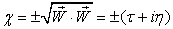
The vector is always called the complex PMD vector. Simply, and vectors represent the PMD and PDL, respectively. The DGD is, while DSA is defined as . It can be shown that the eigenvectors of the matrix are the output principal states of the system (with the PSP definition according to the first order frequency-independent), no matter whether the PDL is zero or not. The eigenvalues of are , which in turns out to be a complex number in systems with PDL. Formally, 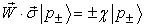. The eigenvectors are orthogonal in systems without PDL because the matrix is Hermitian, whereas the Hermitian property is lost and in turn the orthogonality is not hold anymore in presence of PDL. This means that the PSPs in Stokes space 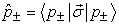are no longer antipodal. Moreover, owing to the traceless of , its two eigenvalues can be written as .

Appendix B

Using the definitions and , one may be found

(B.1)

where

(B.2)

(B.3)

(B.4)

(B.5)

Depending on the Eqs.(B.1) to (B.5), there are many important results that may be specified as follows: if and are parallel or anti-parallel, then and . In turn,

(B.6)

That is; the parallel and anti-parallel cases will present a different orientation of the PSPs without holding the orthogonality. If and are orthogonal, then , and . Consequently,

(B.7)

That is; the DSA will be zero and the DGD will be maximum. Moreover, if we take, then the simplest case that makes (), i.e. which are orthogonal, will be deduced. The absence of PMD effects will make , , and and consequently ,which is a trivial case that means no PSPs states.

For each section there are a local complex vector that may be determined depending on and . In other words, for each section does not depend on the other sections effect, but the total after sections results from the contribution of all transmission matrices of the previous sections. Accordingly, the following facts for the physical parameters of the individual sections may be pointed: , , (the eigenvalues are real), and

(B.8)

That is; the orthogonality is hold at each section if or . As such, the individual PDL effects on the orthogonality will be discarded if no PDL or and are parallel or anti-parallel. Also, if then and , such that the DGD will not change, i.e. . However, all fiber properties depend on the geometrical relation between the local vectors and of each section.

Appendix C

The derivative and inverse of are illustrated as

(C.1)

(C.2)

The frequency derivative of each may be computed using Equation.(3) to show

(C.3)

References

[1]	N. Gisin and B. Huttner, “Combined effects of polarization mode dispersion and polarization dependent losses in optical fibers”, Optics Communications, 142, 119-125, 1997.
	In article		CrossRef PubMed
[2]	N. Gisin, B. Huttner and N. Cyr, ”Influence of polarization dependent loss on birefringent optical fiber networks”, Optical Fiber Communications, 2000.
	In article		CrossRef PubMed
[3]	B. Huttner, C. Geiser and N. Gisin, “Polarization-induced distortions in optical fiber networks with polarization-mode dispersion and polarization-dependent losses”, IEEE J Selected Topics in Quantum Electronics, 6(2), 317-329, 2000.
	In article		CrossRef PubMed
[4]	I. Yoon and B. Lee, "Change in PMD due to the combined effects of PMD and PDL for a chirped gaussian pulse", Opt Express, 12(3), 492-501, 2004.
	In article		CrossRef PubMed
[5]	J. Gordon and H.Kogelnik, "PMD fundamentals: polarization mode dispersion in optical fibers",Proc Natl Acad Sci, 97(9), 4541-50, 2000.
	In article		CrossRef PubMed
[6]	C. D. Poole and R. E. Wagner, “Phenomenological approach to polarization dispersion in long single-mode fibers”, Electronics Letters, 22(19), 1029-1030, 1986.
	In article		CrossRef PubMed
[7]	L. Chen L, Z. Zhang and X. Bao, "Combined PMD–PDL effects on BERs in simplified optical system: an analytical approach", Opt Express, 15(5), 2106-19, 2007.
	In article		CrossRef PubMed
[8]	M. Shtaifand O. Rosenberg, "Polarization dependent loss as a waveform distortion mechanism and its effect on fiber optic systems", JLightwaveTech, 23(2), 923-30, 2005.
	In article		CrossRef PubMed
[9]	Y. Li and A. Yariv, “Solutions to the dynamical equation of polarization-mode dispersion and polarization-dependent losses”, J Optical Society of America. B, 17(11), 1821-1827, 2000.
	In article		CrossRef PubMed
[10]	G.P. Agrawal, “Lightwave Technology”, Wiley-Interscience, 2005.
	In article		CrossRef PubMed
[11]	D. S. Waddy, L. Chen, X. Bao and D. Harris, “Statistics of relative orientation of principal states of polarization in the presence of PMD and PDL”, Proceedings of SPIE, 5260, 394-396, 2003.
	In article		CrossRef
[12]	M. Wang, T. Li and S. Jian, “Analytical theory of pulse broadening due to polarization mode dispersion and polarization dependent loss”, Optics Communications, 223, 75-80, 2003.
	In article		CrossRef PubMed
[13]	C. Xie and L. F. Mollenauer, “Performance Degradation induced by polarization-dependent loss in optical fiber transmission systems with and without polarization-mode dispersion”, J Lightwave Tech, 21(9), 1953-1957, 2003.
	In article		CrossRef PubMed
[14]	S. Yang, L. Chen and X. Bao, “Wavelength dependence study on the transmission characteristics of the concatenated polarization dependent loss and polarization mode dispersion elements”, Optical Engineering, 44(11), (115006) 1-5, 2005.
	In article		CrossRef PubMed