Abstract

This paper considered a long term electric power load forecast for twenty years (20 years) projection, in Nigeria power system using least-square regression and exponential regression model. The model is implemented in Matlab platform with a plot in residential load demand, commercial load demand and industrial load demand in (MW). In the quest for analysis and predicting the energy (power) demand (MW) requirement for a projection period of (2013 - 2032), data are collected between (2000 - 2012), from the Central Bank of Nigeria (CBN), and National Bureau of statistics (NBS). The results obtained shows that energy generated from the respective generating station including Egbin thermal power station Lagos, Sapele thermal power station etc. are grossly inadequate. This mismatch is a major problem in power system planning and operation. The result also shows that there is deviation between predicted energy demand (MW) and available power (or capacity allocated). The predicted energy demand into the projected future of 20years is 45 5,870.2MW. The paper work also extended the prediction form into: least-square, exponential regression model. Evidently, the comparism plot for linear and exponential model which shows similar predicting pattern: particularly least-square exhibit linear behavior, while exponential shows non-linear behaviour, the linear model gives more accurate result as compared to the exponential.

1. Introduction

The generating section are strategically located across the geopolitical-zone in Nigeria with different generating station capacity, people gradually drift from rural to urban cities which has led to an excessive demand of electricity due to the fast growing rate of industries, economic development and increasing population of the residence which has also led to epileptic power supply, power failure, fluctuation and total power outage. It has brought to a loss of energy utilization by the consumers and utility companies.

Peak load forecasting play major role in electrical power system operation, unit commitment and energy scheduling (Amin-Naseri and Soroush, 2008). Energy demand forecasting presents the firsts step in planning and developing for future generation, transmission and distribution facilities. One of the primary tasks of electric utility is to accurately predict energy demand requirements at all times, especially for a long term planning.

Based on the outcomes of such forecasts utilities coordinates their resources to meet the forecasted energy demand, thereby engaging a least-cost Energy management plan and follow-up which are subject to numerous uncertainty that is, in planning for future capacity resource needs an information and operation of the existing generation resources, in order to predicts future capacities and the power system serves one main function that is, to supply energy to the respective customers, which are residential, commercial and industrial consumers with electrical energy as economically and reliable condition. Another responsibility of power utilities is to recognize the needs of their customers Demand and the supply the necessary energies.

Evidently, limitations of energy resources in additions to environmental factors, requires electric energy to be used, more efficiently power plant and transmission lines to be constructed.

1.1. Aim of this Paper

The aim of this paper is to conduct the analysis of the load forecast and energy demand.

1.2. Objectives of this Paper

(i). The objective of this paper is to carry out using engineering techniques, to analyze the behaviour of the energy demand forecast with the aid of data collection.

(ii). To investigate Energy demand profile of the existing capacity and the energy consumption pattern

(iii). To analyse and forecast the energy demand response for a projection of 25 years ahead.

(iv). To recommends to the regulatory agencies for implementing mismatches between the load allocations and the required capacity.

The study shall consider the consumption pattern for residential, commercial and industrial Energy demand forecast, for a projection of twenty-five years ahead.

1.3. Significance of the Paper

The contents of this paper will be of great benefits particularly, to the electricity utilities, regulatory agencies and Nigeria at large, owing to the fact that development of electricity infrastructure is undoubtedly a capital intensive project that needs a serious attention. Hence, Energy demand forecast shall be taken as the first priority for future expansion planning program. Therefore to keep Nigeria abreast with other developing countries which have exhibited in every standard a substantial growth in economic development this means that, the existing gap between the electric power generation and energy demand requirement must be bridged.

2. Problem Statement

Sustainable supply of electric power is a prerequisite for energy generation, transmission and distribution to foster all forms of Economic development in the country. The Nigerian power system is not generating enough electric power, this inadequacy has led to:

(i) Extra ordinary line losses,

(ii) Load shedding,

(iii) Failure and collapse of power system,

(iv) Reduction in quality of electric power

Therefore there is need to overcome this challenges of poor supply of power to the end users at all times.

3. Material and Method

3.1. Least Square

The materials required for the analysis of electricity (demand) prediction in this paper is the load-capacity (allocation) and capacity-utilization data of previous years from Central Bank of Nigeria (CBN), National Beaureau of Statistics (NBS) and Power Holding Company of Nigeria (PHCN).

The paper strongly need to investigate the deviation of the capacity allocated to that of the capacity utilization on the view to analyse the rate of load consumption pattern with respect to capacity allocation by the Central Controlling Body: National Control Centre of Nigeria.

The analysis of demand forecasts are required for expansion, controlling and scheduling of power systems. The forecast help in determining the optimal-mix of generating capacities and which power plant to operate in a given period, so as to minimize costs and secure demand. The study is essential to be able to predict/forecast the quantity of power needed by Nigeria owing to the declining nature of the Nigerian power system supply and plan for future network expansion, in order to reduce cost of energy generation, stop load shedding and reduce power outages to minimum. Energy consumption data are collected for resident, commercial and industrial:

Calculation and Analysis using Parabola (2^nd degree polynomial)

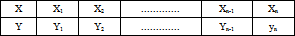
This method employs the least-square technique used in developing a curve that describes the relationship between two or more variables. For example, capacity allocation (A), capacity utilization (U), and difference between the two capacities as errors (E) etc.

That is a given pair of polynomial data can be represented between two sets as:

(3.1)

This can be represented in other form as:

(3.2)

On summing up the columns (equation. 3.2) we have:

(3.3)

The above equation from the basis for the least-square method of 2^nd – degree polynomial curve fit. Considering (equation 3.3), their increasing order of sequences, it can be placed in matrix formation e.g. Hence multiplying equation (3.3) by x:

(3.4)

• Multiply (3.4) by x:

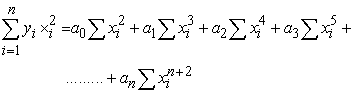(3.5)

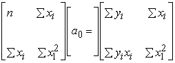
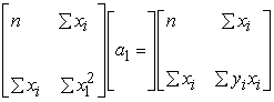
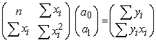
Hence, in matrix form:

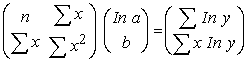
(3.6)

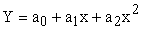
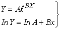
Since the equation of a straight line:

(3.7)

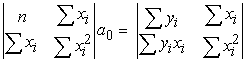
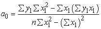
This can be obtained using, determinate by matrix operation; using Crammer rule:

(3.8)

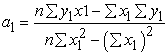
Similarly,

(3.9)

This means that,

(3.10)

Several methods or techniques are usually used and applied in the analysis of load forecasting for energy demand. The research work rely on the least-square and exponential regression techniques this is because of its numerous advantages, measurements error problems, the issues of large variation of data collection, missing observation of data etc. Therefore this work will consider the comparison between the two techniques that is preferred in the analysis.

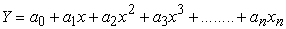
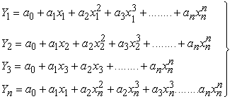
The least square method is one of the mathematical tools used in developing a curve that describe the relationship between two variables. A polynomial of any degree can be established using least square method including the straight line form. A given pair of data can be represented by a polynomial that can best fit the relationship between two set of values, as given in the Table 2.

(3.11)

If the above polynomial fits the pair of data, it means that every pair of data will satisfy the equation (polynomial).

(3.12)

(3.13)

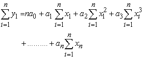
Summation of the sign () with i = 1.

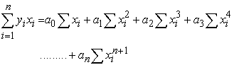
Multiplying equation 3.13 by x_i, we obtain.

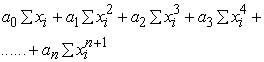(3.14)

Multiplying 3.14 by x_i, we obtain

(3.15)

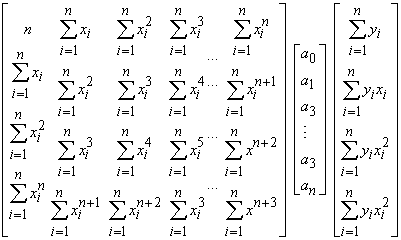
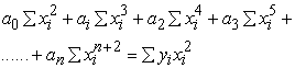
For the nth time, the expression will be:

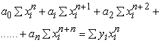(3.16)

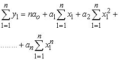
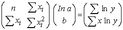
(n + 1) equation. In matrix form, this becomes

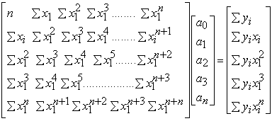(3.17)

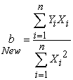
We can now use the least square expression obtained in approximating the relationship between two variables using polynomial of any degree.

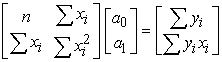
We can use the above expression 3.18 to approximate a straight line equation by extracting 2 2 matrix from the main matrix as shown below:

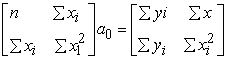(3.18)

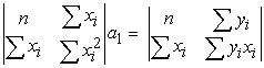
The equation of a straight line is given by y = a₀ + a₁x. We can apply any adequate method in solving the two equations in expression 3.18 to get the values of a₀ and a₁.

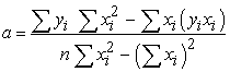
Applying crammer’s rule, this becomes:

(3.19)

(3.20)

(3.21)

(3.22)

The polynomial of the second degree (quadratic equation) can be determined in a similar manner. The matrix formation for such is given as:

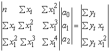(3.23)

The matrix is 3 x 3 since the polynomial of the second degree is of the form

(3.24)

Commercial Demand

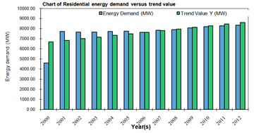
This analysis and procedure is repeated in the same manner for the case of residential and industrial load demand forecast.

The gradient of the trend line

Trend line value when x = 0: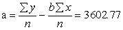

Trend equation

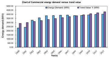
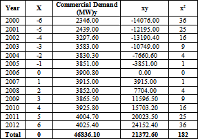
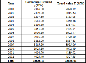
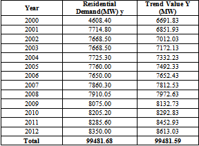
The trend values from the above equation gives the values actual commercial demand and is given in the table below:

• To calculate the accuracy of commercial forecast

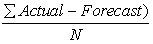
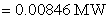
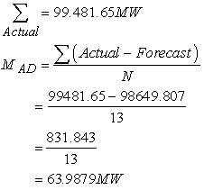
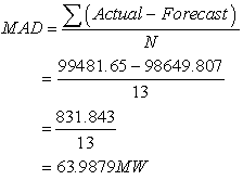
The mean absolute deviation (MAD) = = 0.00692 MW

• To calculate the accuracy of residential forecast

The mean absolute deviation (MAD) = = 0.09/13= 0.00692

• The Predicted Residential Demand

The forecast value can be determined by adding the trend line value (160.10MW) to the preceding load demand to get the current years forecast demand also by using the trend equation.

The gradient of the trend line

Trend equation

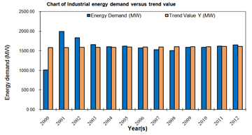
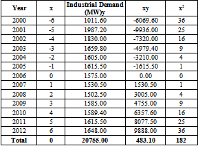
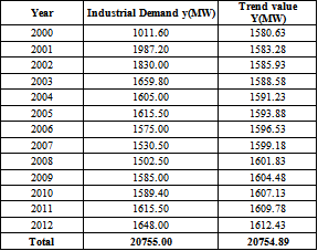
The trend values and actual industrial demand are shown in Table 7 below;

• To calculating the accuracy of industrial forecast

The mean absolute deviation (MAD)

=

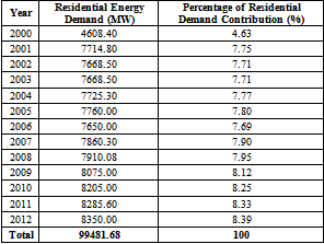
Year 2000: 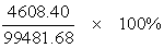=4.63%

Year 2001: 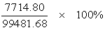=7.75%

Year 2002: 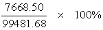= 7.71%

Year 2003: =7.71%

Year 2004: 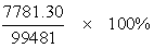=7.77%

Year 2005: 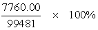=7.80%

Year 2006: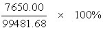 =7.69%

Year 2007: 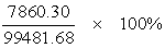=7.90%

Year 2008: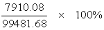 =7.95%

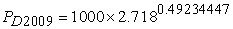
Year 2009: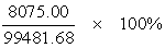 =8.12%

Year 2010: 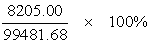=8.25%

Year 2011: 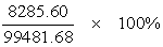=8.33%

Year 2012: 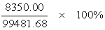=8.39%

Regression Exponential Analysis Method

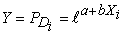
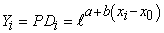
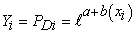
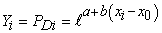
In the case of least-square method, approximation are conducted between two variables, using polynomial of any degree (linear, quadratic, cubic etc). The two variables are expected to fit the function to the set of data, when the predication equation is given as:

(3.7)

Where:

= specify intercepts

= specific slope

= specify dependent variable

= independent variable

The estimated trend value for a given period t,

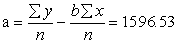
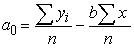
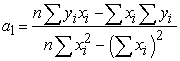
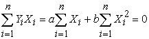
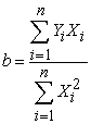
By the application of least square regression through Crammers rule, the constants, a and b can be determined from equation (3.25)

(3.25)

Which are obtained from the matrix formation as:

(3.26)

or

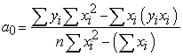(3.27)

or

(3.28)

Similarly,

(3.29)

or

(3.30)

or

(3.31)

The least-square method is used in fitting trend line to a time series. The technique is one of the basic tools used in developing a curve that describes the relationship between variables. This technique can be applied to any n-degree polynomials.

• Exponential Regression Analysis

Considering the curve behaviour, while plotting capacity allocation, capacity utilization and error, the curve of the data trend is non-linear in nature. Therefore there is need to apply the non-linear model: Exponential regression model which can give a good result between the exponential relationship of the variables considered in the study.

This is the therefore achieved by estimating the base-load and the annual growth rate, given as:

(3.32)

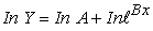
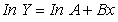
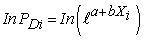
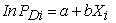
Converting equation (3.32) to a straight line on (linear), we take a rational logarithms of both sides of equation (3.32).

That is,

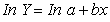(3.33)

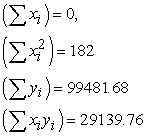
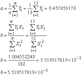
To solve ‘a’ and ‘b’, make a summation to both sides,

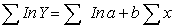(3.34)

Multiply, equation (3.34) by variable “x”

Hence

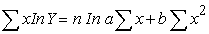(3.35)

From equation (3.34) and (3.35) form your matrix-function trough crammer’s rule, we have:

(3.36)

3.2. Using Exponential Regression Analysis Method

• To determine the values of ‘a’ and “b” respectively, according to the given equations.

Substituting, the values obtained in the Table 9 into equation (3.36)

(3.36)

Where:

(3.37)

(3.38)

The system equation becomes:

(3.39)

(3.40)

or

(3.41)

(3.42)

or

(3.43)

(3.44)

(3.45)

(3.46)

Therefore,

(3.47)

or

(3.48)

(3.49)

But,

(3.50)

Therefore,

(3.51)

Hence, substituting the values of “a” and “b” into the equation as:

(3.52)

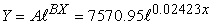
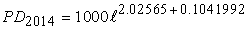
Where, “b” is the growth rate is obtained from equation (3.52) as:

(3.53)

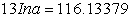
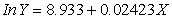
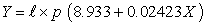
But, slope is the antilog of the value (0.02423) = 1.02452

Hence,

(3.54)

Therefore, b = growth rate = 2.5%

(3.55)

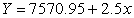
This means substituting values of “x” into the relation y = a + bx to obtain other value of y.

The predicted load “Y”, using exponential regression function are presented as:

, the predicted value will be:

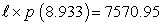
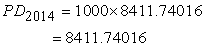
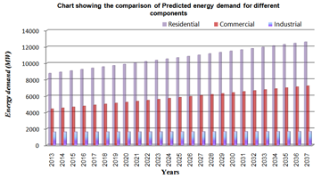
For 2013 - New predicted value (MW) = 7570.95 + 189.2738 = 7769.22MW

For 2014 - New predicted value (MW) = 7760.22 + 189.2738 = 7949.497MW

For 2015 - New predicted value (MW) = 7949.498 + 189.2738 = 8138.7718MW

For 2016 - New predicted value (MW) = 8138.7718 + 189.2738 = 8328.0456MW

For 2017 - New predicted value (MW) = 8328.0456 + 189.2738 = 8517.319MW

For 2018 - New predicted value (MW) = 8706.5932MW

For 2019 - New predicted value (MW) = 8706.5932 + 189.2738 = 8895.867MW

For 2020 - New predicted value (MW) = 8895.867 + 189.2738 = 9085.1408MW

For 2021 - New predicted value (MW) = 9085.1408 + 189.2738 = 9274.4146MW

For 2022 - New predicted value (MW) = 9274.4146 + 189.2738 = 9463.6884MW

For 2023 - New predicted value (MW) = 9463.6884 + 189.2738 = 9652.9622MW

For 2024 - New predicted value (MW) = 9652.9622 + 189.2738 = 9842.236MW

For 2025 - New predicted value (MW) = 9842.236 + 189.2738 = 10031.5098MW

For 2026 - New predicted value (MW) = 10031.5098 + 189.2738 = 10220.7836MW

For 2027 - New predicted value (MW) = 10220.7836 + 189.2738 = 10410.0574MW

For 2028 - New predicted value (MW) = 10410.0574 + 189.2738 = 10599.3312MW

For 2029 - New predicted value (MW) = 10599.3312 + 189.2738 = 10788.605MW

For 2030 - New predicted value (MW) = 10788.605 + 189.2738 = 10977.8788MW

For 2031 - New predicted value (MW) = 10977.8788 + 189.2738 = 11167.1526MW

For 2032 - New predicted value (MW) = 11167.1526 + 189.2738 = 11356.4264MW

Predicted load (Y) in the case of using least-square method

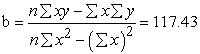
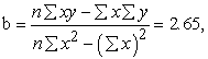
The gradient of the trend-line:

Where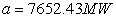

b = 160.10 (which is 2.092% of the growth rate)

That is,

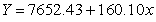
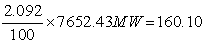
=160.10MW (capacity addition)

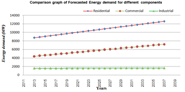
For 2013 - New predicted value: = 7652.43 + 2.093% 1 = 7812.53MW

For 2014 - New predicted value: = 7652.43 + 2.093% 2 = 7972.63MW

For 2015 - New predicted value: = 7652.43 + 2.093% 3 = 8132.73MW

For 2016 - New predicted value: = 7652.43 + 2.093% 4 = 8292.83MW

For 2017 - New predicted value: = 7652.43 + 2.093% 5 = 8452.93MW

For 2018 - New predicted value: = 7652.43 + 2.093% 6 = 8613.03MW

For 2019 - New predicted value: = 7652.43 + 2.093% 7 = 8773.13MW

For 2020 - New predicted value: = 7652.43 + 2.093% 8 = 8933.23MW

For 2021 - New predicted value: = 7652.43 + 2.093% 9 = 9093.33MW

For 2022 - New predicted value: = 7652.43 + 2.093% 10 = 9253.43MW

For 2023 - New predicted value: = 7652.43 + 2.093% 11 = 9413.53MW

For 2024 - New predicted value: = 7652.43 + 2.093% 12 = 9573.63MW

For 2025 - New predicted value: = 7652.43 + 2.093% 13= 9733.73MW

For 2026 - New predicted value: = 7652.43 + 2.093% 14 = 9893.83MW

For 2027 - New predicted value: = 7652.43 + 2.093% 15 = 10053.93MW

For 2028 - New predicted value: = 7652.43 + 2.093% 16 = 10214.03MW

For 2029 - New predicted value: = 7652.43 + 2.093% 17 = 10374.13MW

For 2030 - New predicted value: = 7652.43 + 2.093% 18 = 10534.23MW

For 2031 - New predicted value: = 7652.43 + 2.093% 19 = 10694.33MW

For 2032 - New predicted value: = 7652.43 + 2.093% 20 = 10854.43MW

Modified form of Exponential Regression Analysis

(3.56)

(3.57)

or

(3.58)

Therefore the modified form of exponential demand equation may be expressed as:

(3.59)

or

(3.60)

Where :

becomes;

(3.61)

Now, taking natural log of equation (3.5):

We obtain as:

(3.62)

or

(3.63)

or

(3.64)

Where:

(3.65)

The utilization load demand is represented as expected demand while allocated load is represented as available power (MW):

For considering the historical data for energy demands for consecutive year are

(3.66)

(3.67)

(3.68)

• In order to predicts the demand correctly, the sum of square of error should be minimum:

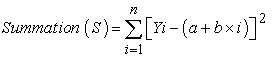(3.69)

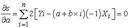
• For S to be minimum, the conditions are:

(3.70)

Differentiating equation (3.14) with respect to 'a' we have:

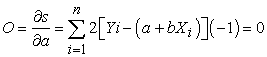or

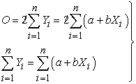(3.71)

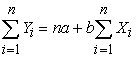(3.72)

• Similarly, differenting equation 3.14) with respect to 'b' we have:

(3.73)

or

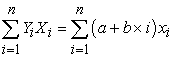(3.74)

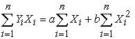(3.75)

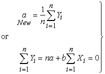
• Hence, the conditions for the sum of least square of the error (deviation), to be minimum are given by the two equations:

Let us consider

(3.76)

in order to determine ‘a’ and ‘b’

• Using the equation (3.21) into equation (3.17) and (3.20) :

We have:

(3.77)

or

Similarly,

or

(3.78)

or

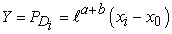
• Hence for load prediction we have:

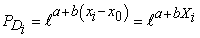(3.79)

Where:

= 2.718

: intercept

: slope or gradients

: projected look ahead period

: difference between projected year and base year (MW)

: base year (reference year) = 2006

: base – MW =

where:

where

and

Modified Form of Exponential Regression Calculation and Analysis for load demand for the year 2013, when our base year is equal 2006
Case 1: Residential

Where

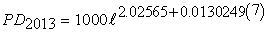
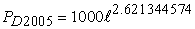
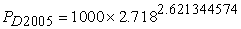
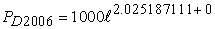
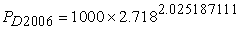
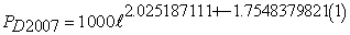
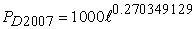
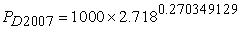
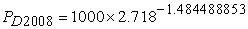
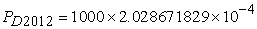
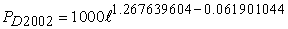
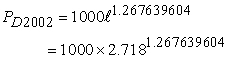
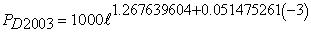
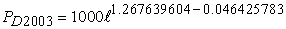
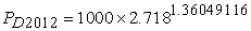
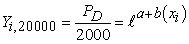
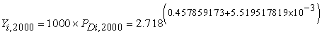
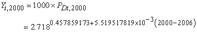
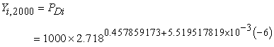
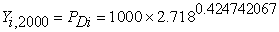
But = predicted energy demand = 2013.

= based - year = 2006

Note:

We can find our peak load demand from

But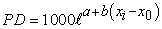

That is when =2006 (datum case) or base year

=2013 (prediction case)

Hence;

or

Modified Form of Exponential Regression Calculation and Analysis For load demand for the year 2014, when our base year is equal 2006

That is;

When =2006 (datum case) or base year

=2014 (prediction case)

Therefore;

But

This process is continued in the same similar manner

Total summation of predicted load in the case of residential load (2000 – 2012)

That is,

∑ predicted residential energy demand = (7009.723+7101.6150 + 7194.708 + 7289.02 + 7384.571 + 7481.37 + 7579.44+7678.80 + 7779.46+7881.44 +7984.76+ 8089.43+ 8195.47)

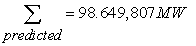Similarly, the actual allocated Residential load between (2000 – 2012) becomes:

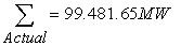
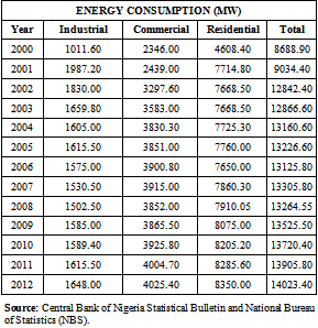
∑_Actual = (4608.40+7714.80 + 7668.50 + 7668.50 + 7725.30 + 7760.00 + 7650.00 + 7860.30 + 7910.05 + 8075.00 + 8205.20 + 8285.60 + 8350.00) =

Case 1: Validation: Residential load demand

Capacity Allocation @ 2000 = 4608.40MW (or available)

Load forecast (prediction) @ 2000;

Where

= base year = 2006

= predicted year = 2000

@ 2001 (Prediction)

or

or

or

@ 2002 (Prediction)

or

or

or

or

or

@ 2003 (Prediction)

or

or

or

or

or

@ 2004 (Prediction)

or

or

or

or

or

@ 2005 (Prediction)

or

or

or

or

@ 2006 (Prediction)

or

or

or

or

or

@ 2007 (Prediction)

or

or

or

or

@ 2008 (Prediction)

or

or

or

or

or

@ 2009 (Prediction)

or

or

or

or

@ 2010 (Prediction)

or

or

or

or

or

or

@ 2011 (Prediction)

or

or

or

or

or

@ 2012 (Prediction)

or

or

or

or

or

Total summation of predicted load in the case of Residential load (2000 – 2012)

That is,

∑ Predicted Residential energy demand = (7009.723+7101.6150 + 7194.708 + 7289.02 + 7384.571 + 7481.37 + 7579.44+7678.80 + 7779.46+7881.44 +7984.76+ 8089.43+ 8195.47)

Similarly, the actual allocated Residential load between (2000 – 2012) becomes:

∑_Actual = (4608.40+7714.80 + 7668.50 + 7668.50 + 7725.30 + 7760.00 + 7650.00 + 7860.30 + 7910.05 + 8075.00 + 8205.20 + 8285.60 + 8350.00) =

Standard Error Predication

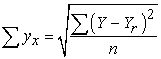
Standard error of prediction

Analysis of Allocation (Available demand) in MW wrt to energy demand prediction (forecast)

Where

Where Predicted Energy Demand

= base year = 2006

= 2000

= 2.718

= base year (Reference year) 2006

B = base – MW = 110³ =1000MW

Commercial Demand

Capacity allocation @ 2000 = 2346.00 (or available)

Load forecast (prediction) @ 2000

Where

= base year = 2006

Predicted year = 2006

2001 (Prediction)

2002 (Prediction)

2003 (Prediction)

2004 (Prediction)

2005 (Prediction)

2006 (Prediction)

2007 (Prediction)

2008 (Prediction)

2009 (Prediction)

2010 (Prediction)

2011 (Prediction)

2012 (Prediction)

Total summation of predicted load in the case of Commercial load (2000 – 2012)

That is,

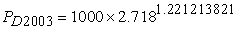
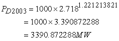
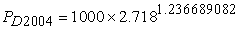
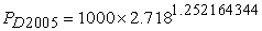
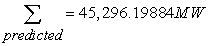
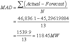
∑ Predicted Commercial energy demand = 2608.273809 + 2746.036366 + 3551.990568 + 3390.872288 + 3443.749528 + 3497.451339 + 3551.990568 + 3607.380282 + 3663.633742 +3720.764419 +3778.785991 + 3837.71235 + 3897.557592 = 45,298.19884MW

Similarly, the actual allocated Commercial load between (2000 – 2012) becomes:

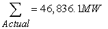
∑_Actual = 2346.00 + 2439.00 + 3297.60 + 3583.00 + 3830.30 + 3851.00 + 3900.80 + 3915.00 + 3852.00 + 3865.50 + 3925.80 + 4004.70 + 4025.40 = 46, 836.1MW

INDUSTRIAL DEMAND

Analysis of Allocation (Available demand) in MW wrt to energy demand prediction (forecast)

Where

Where Predicted Energy Demand

= base year = 2006

= 2000

= 2.718

= base year (Reference year) 2006

B = base – MW = 110³ =1000MW

Capacity allocation @ 2000 = 1011.60 (or available)

Load forecast (prediction) @ 2000

Where

= base year = 2006

Predicted year = 2006

2001 (Prediction) Industrial Demand

2002 (Prediction) Industrial Demand

2003 (Prediction) Industrial Demand

2004 (Prediction) Industrial Demand

2005 (Prediction) Industrial Demand

2006 (Prediction) Industrial Demand

2007 (Prediction) Industrial Demand

2008 (Prediction) Industrial Demand

2009 (Prediction) Industrial Demand

2010 (Prediction) Industrial Demand

2011 (Prediction) Industrial Demand

2012 (Prediction) Industrial Demand

Total summation of predicted load in the case of Industrial load (2000 – 2012)

That is,

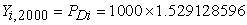
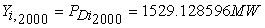
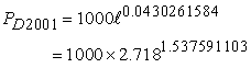
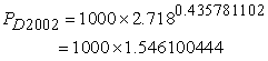
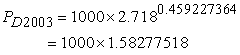
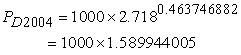
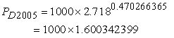
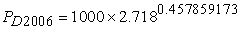
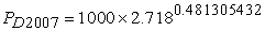
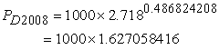
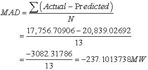
∑ Predicted Commercial energy demand = 1529.128596 + 1537.591103 + 1546.10044 + 1582.77518 + 1589.944005 + 1600.342399 + 1609.199074 + 1618.104703 + 1627.058416 + 1636.064105 + 1645.118416 + 1654.222836 + 1663.377641 = 20,839.02692MW

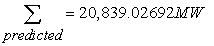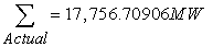
Similarly, the actual allocated Commercial load between (2000 – 2012) becomes:

∑_Actual = 1011.60 + 1987.20 + 1830.00 + 1659.80 + 1605.00 + 1615.50 + 1575.00 + 1502.50 + 1585.00 + 1589.40 +1615.50 + 1648.00 = 17,756.70906MW

OW CHART SHOWING THE ACTIVITIES OF LEAST AND EXPONENTIAL REGRESSION ANALYSIS

4. Results and Discussion

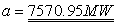
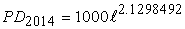
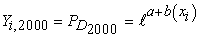
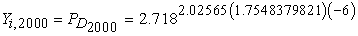
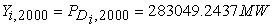
The maximum load calculated with exponential regression, function is given as: 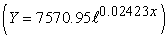with percent growth rate of 2.5%, while the maximum load calculated for least-square regression function is given as: with growth rate of 2.093%. Therefore the maximum load: (7570.95MW) with 2.5% growth rate from exponential regression analysis method is more realistic and appropriate because of its ability to capture the energy requirement for consumers at the receiving end, on the view with steady energy growth-rate.

Load forecasting analysis is a major problem in power system planning and operations. This is because it provides then necessary information for: customer service and billing, electricity pricing and tariff planning etc. thereby giving an insight into future expansion planning.

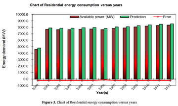
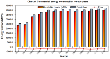
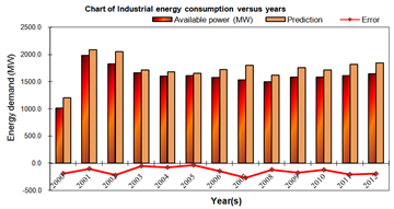
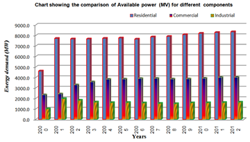
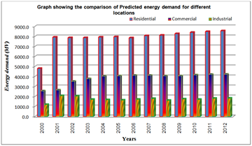
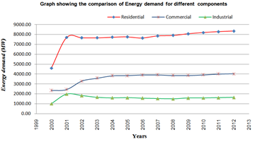
The result obtained shows that the utilization capacity (MW) does not give positive reflection of the capacity allocations (MW) when conducted in Matlab/Java platform especially in the case of residential, commercial and industrial plot (MW).

This mean that there is a deviation between installed capacity and that of utilization capacity of the consumer at the receiving end which need to be match in order to avoid overload and system collapse.

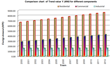
The paper work also extended to the linear model (lgast-square regression) and exponential regression plot which exhibit and confirms similar relationship in residential, commercial and industrial plot.

Evidently, the comparism plot for linear model and exponential regression show different behaviour, the least square model display linear graph while the exponential graph exhibit non-linear behaviour which is recommend because of the nonlinear relations between the capacity allocation (MW) and that of capacity in utilization.

EXPONENTIAL REGRESSION ANALYSIS
LEAST SQUARE REGRESSION ANALYSIS

5. Conclusion

The electricity load forecast is a comprehensive survey of electrical demand and supply at the receiving end, in order to identify areas of inadequacies resulting to mismatches, which may negatively impact an overloads on transmission and distribution network. This work carried out load forecast using the analysis of least-square regression and exponential regression and validated in Matlab and Java programming platform.

Data are collected from (2000 - 2012) Central Bank of Nigeria (CBN) and National Bureau of statistics which serves as the input data into the least-square and exponential regression model for prediction into the projected future 2032. The result obtained shows that there is mismatch between installed capacity (MW) and utilization capacity (MW) in the case of residential, commercial and industrial load demand. Evidently, the result suggested that there is need to bridge the gap in order to enhance high reliability and efficiency in power system operation.

This work also identified the relationship between least-square model and exponential model plot on Matlab and Java program environment. Since the deviation between the installed and utilization capacity (MW) are non-linear, the exponential regression plot is therefore recommended, because of the non-linear behaviour of the capacity and load demand requirement.

Therefore, strategies for expansion programme is required for engaging distribution generator (DG) or decentralized generator via distribution outlet, on the view to solve overloads problems. This suggestion and recommendation if implemented will improve the electricity supply and demand in Nigeria.

6. Recommendation

Owing to the finding obtained in the course of this research the following recommendation are made:

(i) To meet the energy demand requirement, additional capacity generation will be required.

(ii) Additional injection station and substation must be build to cater and care for rapid increase in load demand.

(iii) Generation expansion program must be in place to accommodate annual growth of energy consumption.

References

[1]	Adepoju, G.A., Ogunjuyigbe, S.O.A., Alexiadis, K. O. and Maissis, A. H. (2007)“Along Term Load Forecasting Model for Greek Power Systems” Pacific Journal of Science and Technology. ISS. B Vol, 1 pp. 68-72.
	In article
[2]	Al Mamun M., and Negasaka K. (2004) “Artificial neural networks applied to long-term electricity demand forecasting:” Proceedings of the Fourth International Conference of n Hybrid Intelligent Systems (HIS’04), pp. 204-209.
	In article		View Article
[3]	Amin-Naseri, M. R, Soroush, A. R (2008). Combined use of unsupervised and supervised learning for daily peak load forecasting energy conversion and management, 49(2008) PP1302-1308. Available [online]: www.sciencedirect.com
	In article		View Article
[4]	Atiya A.F. (1996) “Development of at intelligent long-term electrics load forecasting system”, proceedings of the international conference of ISAP apo, pp, 288.
	In article		View Article
[5]	Ayesha Afzaal,Mohsin Nazir, Ayesha Ali, and Aneeqa Sabah (2015) “Green Net: Agent based Energy Load Prediction Techniques for Smart Grid” pp. 27-33.
	In article		View Article
[6]	Bakirtzis, A.G. V., Petridis, S. J., Kiartzis, Alexiadis, M.C. and Maissis, A. H. (1996) “A Long Term Load Forecasting Model for Greek Power System”, IEEE transactions on Power systems, 11pp. 858-863.
	In article
[7]	Bansal, R.C. and J.C. Pandey, 2005. Load forecasting using artificial intelligence techniques: A literature survey. Int. J. Comput. Appli. Technol., 22: 109-119.
	In article		View Article
[8]	Bansal, R.C. and J.C. Pandey, 2005. Load forecasting using artificial intelligence techniques: A literature survey. Int. J. Comput. Appli. Technololgy., 22: 109-119.
	In article		View Article
[9]	Brown, R.E. and J.W. Taylor, 2001. Electric power distribution reliability and network load forecasting. IEEE Trans. Power Syst., 17: 662-672.
	In article
[10]	Cancelo, JR. and A. Espasa, 1991. Forecasting daily demand for electricity with multiple-input nonlinear transfer function models: A case study. Working Paper 91-21, Departamento de Economia, Universidad Carlos III de Machid, Spain, July 1991, pp: 1-73.
	In article		View Article
[11]	Carmona D., Jaramillo M. A., Gonzalcz E. And alvarez A. J. (2002) ‘Electric energy demand forecasting with neural networks’, IEEE, 28TH Annual C. reference of the industrial Electronics society, Vol. 3 pp. 1860-1865.
	In article		View Article
[12]	Dang Khoa T. Q. and Oanh P.T., (2005) “ Application of Elman and neural vavelet network to long –term Load forecasting”, ISEE Journal, track 3, sec. B, No. 20, PP. 1-6.
	In article		View Article
[13]	Eleanya, M.N., Ezechukwu, O.A and Olurum, B. I. (2007) “problems of Transmission and Distribution Network: Nsukka as a test case “international Journal of Electrical & Telecommunication Systems Research (Electroscope), p.p. 126-130.
	In article
[14]	Fu C. W. and Nguyen T. T. (2003) “Models for long-term energy forecasting”, IEEE power Engineering Society General Meeting, Vol. 6, No I,pp 235-239,13-17.
	In article		View Article
[15]	Gellings, C.W., 1997. Demand Forecasting for Electric Utilities. The Fairmont Press, Lilburn, G.A., USA.
	In article		View Article
[16]	Genethliou D. and Feinberg E.A.(2005) Load forecasting, Applied mathematics for restructured electric power system: optimization, control and computational inmelligence (j.H.Chow, F.F. Wu, and J. J. Momoh, eds), chapter 12, pp 269-285.
	In article
[17]	Idoniboyeobu, D.C and Ekanem, M.B (2014) Assessment of Electric Load Demand and Prediction of Future Load Demand: Acase Study of AkwaIbom State of Nigeria, PP 525-535.
	In article		View Article
[18]	Idoniboyeobu, D.C. and G.F. Odubo, 2010. Electrical Load Forecast in Bayelsa State of Nigeria by the year 2020. Niger. J. Ind. Syst. Stud., 9: 22-27.
	In article
[19]	Idoniboyeobu, D.C. and M.A. Newman, 2013. Electric load prediction technique using multiple regression method a case study of Port Harcourt metropolis. Eur. J. Sci. Res., 118: 61-74.
	In article
[20]	IPCL., 2007. Ibom power company annual report, 2007. Ibom Power Company Limited, USA. http:/Iwww.ibompower.net/.
	In article		View Article
[21]	IPCL., 2012. Ibom power company annual report, 2012. Thom Power Company Limited, USA. http://www.ibompower.net/.
	In article		View Article
[22]	Jude, I.E., Micah, E. O, and Edith, N. J. (2005) “Statistics and Quantitative methods for construction and Business Managers” Nigeria institute of building, PP. 1-6, Nigeria
	In article
[23]	Kandil M. S., El- Debeiky S. M. and Hasanien N. E. (2001), ‘The implementation of long-term forecasting strategies using a knowledge –based expert system: part-11’, Electric power system Research (Elsevier), Vol. 58, No.1, pp. 19-25.
	In article		View Article
[24]	Karanta, I. and J. Ruusunen, 1991. Short term load forecasting in communal electric utilities. Research Reports, Helsinki University of Technology, May 1991, Page: 104.
	In article
[25]	Karanta, I. and J. Ruusunen, 1991. Short term load forecasting in communal electric utilities. Research Reports, Helsinki University of Technology, May 1991, Page: 104,
	In article
[26]	Kermanshahi B.S., and Iwamiya h. (2002) “Up to year 2020 load forecasting using neural nets”, Electric power System Research (Elsevier), Vol. 24, No. 9, pp. 739. 797.
	In article		View Article
[27]	Khoa T.Q.D., Phuong I., M., Binh P.T.T. and Lien N. T.H. (2004) “Application of wavelet and neural network to long-term load forecasting”, International Conference on Power System Technology (POWERCON 2004), pp. 840-844, Singapore, 21-24.
	In article		View Article
[28]	Khoa T.Q.D., Phuong L. M., binh P. T. T., Lien N. T. H. (2004) “Power load forecasting algorithm based on recurrent support vector machines with genetic algorithms’ 39th International Universities Power Engineering conference, UPEC 2004, Vol. 1. Pp. 368-372.
	In article
[29]	Labrune, M.P. and J.W. Taylor, 2001. Short term electricity demand using double seasonal exponential smoothing. J. Operat. Res. Soc, 54: 799-805.
	In article		View Article
[30]	Labrune, M.P., and J.W. Taylor, 2001. Short term electricity demand using double seasonal exponential smoothing. J. Operat. Res. Soc, 54: 799-805.
	In article		View Article
[31]	Luciano G.V (2016) “Statistical modeling and forecasting of daily peak electricity load”.
	In article
[32]	Marcel, D. and D.W. Bumn, 2002. Forecasting loads and process in competitive power market. Proc. IEEE., 88: 163-169.
	In article
[33]	Oupta, B.R. (2007) Tower system Analysis and design”, S. Chand & Company Ltd Ram Nager, PP 260-274, New Deihi, Idia.
	In article
[34]	Phimphachanh S., Chamnongthai K., Kumhom P., and sangswang A. (2004) “Using neural network for long term peak load forecasting in vientine municipality”, IEEE Region 10 conference, TENCON 2004, Vol. 3 pp. 319.322.
	In article		View Article
[35]	Sambo, S. A. (2008) “Electricity Demand from customers of INGA Hydropower projects: The case of Nigeria “paper presented at the WEC workshop on Financing INGA Hydropower projects, pp. 21-22, London, U.K.
	In article		View Article
[36]	Stroud, KA. and D.J. Booth, 2001. Engineering Mathematics. 5th Rev. Ecin., Paigrave Macmillan, New York, USA., ISBN-13: 978-0333919392, Pages: 1264.
	In article
[37]	TaradarHeque M. and Kashtiban A. M. (2005) “application of neural networks in power system; Areview”, Transaction of Engineering, 1305-5313, pp -53-57.
	In article		View Article
[38]	Uche, C.C.N. and Joseph, T.C. (2007) Energy Infrastructure in Nigeria and Achievement of Millennium Development Goals By 2015”. Journal of Economic studies Vol. 6.
	In article
[39]	Uhunmwangho, R. and E.K. Okedu, 2008. Electrical power distribution upgrade: Case of towns in Akwa Ibom State, Nigeria. Int. J. Applied Eng. Res., 3: 1833-1840.
	In article		View Article
[40]	Wallnestrom, C.J., 2008. On Risk management of electrical distribution systems and the imp act of regulations. Licentiate Thesis, KTH-Royal Institute of Technology Stockholm, Sweden.
	In article		View Article
[41]	Weedy, B.M., 1979. Electric Power System. 3rd Edn., John Wiley and Sons Australia Ltd., Australia, ISBN-13: 9780471275848, pp: 40-41.
	In article