1. Introduction

In the oil and gas industry, pipeline technology have been in continuous growth since its’ early beginnings in California a century ago ^[1]. Currently, as the offshore pipeline moves into more complex conditions, it encounters several challenges. Pipelines laid on soft seabed undergoes high temperature/high pressure cycles during their lifespan and are prone to damages due to different factors that should be studied. Health monitoring of pipeline systems is an important issue and there is a need to develop some systems like what Champiri et al. developed for marine structures ^{[2, 3]}. One of the phenomena associated with underwater extreme situation is that the pipeline moves axially towards its’ cold end, which is the end of the pipeline farthest away from the well. This axial displacement of the pipeline is called pipeline walking.

Based on Bruton et al. (2008) ^[4], the pipe/soil response is the extreme uncertainty in the design of pipelines prone to walking. Many of the previous studies into pipe/soil interaction have concerned stability under hydrodynamic loading, and not the actual interaction between pipe and soft soil. The focus of pipe/soil interaction becomes more and more significant as subsea pipelines are required to operate at higher temperatures and pressures. This can cause uncontrolled lateral buckling and global axial displacement. To consider these two phenomena, and especially the latter, an accurate modelling of the pipe/soil properties is essential.

The pipe/soil interaction model depends on seabed stiffness and an equivalent friction to represent the soil resisting any movement of the pipe ^[5]. The interaction between pipe and soil is typically modelled by connecting pipe/soil elements in intervals along the pipeline length ^[4]. These elements represent the axial and lateral forces that influence the pipe/soil interaction.

To model the pipe/soil interaction, a simple friction factor was used, although this might represent an over-simplification of the behavior ^[4]. A non-linear force/displacement behavior is thus better to represent pipe/soil behavior. Hence, the maximum resistance was divided by the submerged weight of the pipeline ^[6].

The early solutions for pipe-lay presumed the seabed as rigid, which extremely simplified the pipe–soil interaction problem ^[7]. Such solutions increase the maximum pipe–soil contact force and the curvature at the contact point. Afterward, solutions based on linear elastic seabed response were introduced ^{[8, 9, 10]}. Conventional geotechnical approached have been empirically established using analytical closed-form solutions or empirically derived and regulated from experimental data ^{[11, 12, 13]} based on bearing capacity and frictional simulations, with break-out forces ^{[14, 15]}. On the numerical front, various studies such as ^[16] investigated the similar pipe-soil interaction behavior, using the Coupled Eulerian Lagrangian (CEL) and Arbitrary-Lagrangian-Eulerian (ALE) formulations.

Pipelines laid on ultra- soft seabed due to large movements and lateral buckling show global instability of the entire system and ensuing breaking of the pipelines at crucial locations ^[17]. Hence, it is critical to address the issues regarding ultra-soft soil characterization and axial-pipe soil interaction. Vipulanandan et al. (2013) ^[18], proposed a testing framework for monitoring the axial behavior of pipes on soft soil, based on series of experiments performed on relatively small scale model test. More realistic understanding of the interaction phenomena are guaranteed when the testing framework is scaled up. In this paper, precious characterizing of the ultra-soft soil around the pipeline with high accuracy monitoring technique for pipeline movement, in large-scale realistic setup is discussed. In addition, an analytical model is presented to better predict the axial behavior of pipe soil interaction.

2. Objective

The overall objective of this study was to model the axial pipe-soil interaction behavior in ultra-soft soil using large scale laboratory testing. The specific objectives of this study were as follows:

1. Perform precious large-scale laboratory testing of pipe in ultra-soft soil under axial loading conditions.

2. Predict the shear strength of ultra-soft soil using new models.

3. Develop a new model to predict the full axial force-displacement relationship of pipe in ultra-soft soil.

3. Methods and Materials

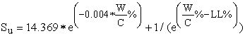
Large-scale model test was used to represent pipe interaction with ultra-soft clay soil simulating the seabed. In this study, it was significant to build an illustrative seabed with appropriate soil strength for the model study. The topography of the seabed is an extra critical concern since the pipes will be deformed and then partially buried in the ultra-soft soil. When the pipe slides on the soil based on the buried depth and movement of the pipe, soil is also moved, berms are formed and higher stresses and deformation appears in the pipe. The experimental setup is presented in Figure 1. Large ultra-soft soil sample with dimension of 2.4 m length, 2.4 m width and 1.8 m height was carefully prepared in order to properly simulate real seabed condition. A displacement controlled machine was used to test the sliding pipe and the pipe was attached to the loading machine with a nonflexible string. In the axial testing, the pipe was pulled with varying rates. A plastic pipe with diameter (D) of 6 cm and thickness (t) of 5 mm was used to represent the insulation surface of the actual pipe. The length of the tested pipe was 1.2 m. To locate soil deformation path during axial loading, three cameras in X, Y and Z directions with Remote Gridding System (RGS) were applied and subsequently; the data from camera were analyzed using Matlab computer program. In order to make the soil deformation noticeable for camera; color flocks were mixed on top of the soil. New Remote Gridding System (RGS) was developed for the first time during this study to assist cameras for better synchronizing pipe movement and soil deformation.

Download as

• PPT
  PowerPoint Slide
• PNG
  Larger image(png format)

Veiw figureFigures index

•  NEW
  View larger figure in new window

View next figure

Figure 1. Axial pipe soil interaction testing facility

Different correlations to predict the undrained shear strength (Su) of soft soil have been reported in the literature ^[19]. The undrained shear strength of soil varied from (0.3 to 25) kPa. The shear strength has been correlated to soil properties such as plastic limit (PL), liquid limit (LL), and water content (W/C) (ratio of weight of water to weight of solid). Based on literature review, over 100 data were collected from different sources for the analyses. New strength relationships were attempted for the very soft soil in terms of moisture content and liquid limit. Therefore, it was very important to re-evaluate some of the correlation equations in the literature and check their effectiveness for predicting the shear strength of soft soil. In addition, new correlations for shear strength in soft soil were introduced combining test results of laboratory miniature vane shear test with high moisture contents and data from the literature. Two relationships are proposed based on the water content and liquid limit of the soft soil ^[20]:

Model 1: Total of 92 data collected from the literature was used to develop this strength relationship. The strength of the soil varies from (1 to 10) kPa.

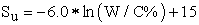(1)

Model 2: Soft soil with varying percentage of bentonite content was used in this study. The clay content varied from (2 to 10) %. The strength of the soil varies from (0.1 to 1) kPa.

(2)

where Su is the undrained shear strength of the ultra-soft soil, W/C is the moisture content, and LL is the liquid limit.

The resistance to pipe sliding on the ultra-soft soil was observed using a load cell (Figure 1). The load cell was regulated to an accuracy of 0.005 N. The pipe displacement in vertical and horizontal directions was monitored with two sets of linear variable differential transducers (LVDT).

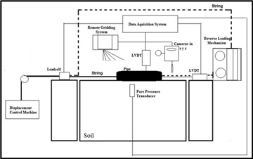
Remote Gridding System (RGS) is composed of a projector and series of transparent grids that are reflected on the surface of model test. Set of three cameras are positioned along x, y and z axes to capture soil displacement at desired area at any time. To make the soil displacement visible for camera, specific color chips were placed on top layer of soil. RGS assists cameras to better synchronize pipe movement and soil deformation at any time increment (Figure 2).

Download as

• PPT
  PowerPoint Slide
• PNG
  Larger image(png format)

Veiw figureFigures index

•  NEW
  View larger figure in new window
• PREV
  View previous figure

View next figure

Figure 2. Schematic of the axial sliding testing setup

To apply RGS precisely, the following steps are required:

1- Collect the RGS pattern sheets by copying the gridlines (from a calibrated parent model outside the soil tank) to transparent sheets. These transparent sheets are then placed on the projector and reflected on the soil model. The angle and distance of projector should be aligned in a way to form 5 cm by 5 cm squares on the whole surface of soil model.

2- Adjusting and regulating the change in the shape and angles of reflected grids to the new topography of soil in every square. Suppose “pattern 1” is reflected on the soil model and due to pipe movement, one or some of the gridline squares turn into “shape A”. By a quick predict, it is clear that this new gridline represent a decrease in the elevation of soil in that area or a puddle ; but the major challenge is to quantitatively relate any change in the angle or configuration of gridline to the new topology of model. To address this challenge, different topography of soil with different slops were constructed in the laboratory and new gridline patterns meticulously photographed and recorded to make a database.

3-Locating disk-shaped, light-weighted color chips (with diameter of 6 mm) on the surface of soil model before starting the test. As the test proceeds, these very small chips will move with particles of ultra-soft soil (undrained shear strength of 0.01 to 0.1 kPa) and for choosing distinct colors, they are easier to be tracked. This step is highly recommended if displacement fields in the soil surface are required.

4-Performing the test and recording pipe and soil movements from three cameras in x, y and z axes simultaneously.

5- For any time increment, the photos should be examined and nodes (grids intersection) in each photo should be appointed to mathematical coordinates using computer programs (Auto desk Maya 2011 and Matlab 2012 Ra). Berms and heaves geometry is closely evaluated by merging coordinates of nodes from X, Y, Z cameras (Figure 3 and Figure 4).

Download as

• PPT
  PowerPoint Slide
• PNG
  Larger image(png format)

Veiw figureFigures index

•  NEW
  View larger figure in new window
• PREV
  View previous figure

View next figure

Figure 3. RGS application on real laboratory test

Download as

• PPT
  PowerPoint Slide
• PNG
  Larger image(png format)

Veiw figureFigures index

•  NEW
  View larger figure in new window
• PREV
  View previous figure

View next figure

Figure 4. RGS simulation for axial full scale testing

4. Modeling

The classical undrained method to define the axial resistance capacity of pile shaft in cohesive soils known as total stress “alpha method” are widely used where axial force is computed as a product of the shear strength Su, the contact area between the pipe-soil Ai and a factor named α dependent on the pipe surface roughness. It is assumed that after the breakout, the shear strength reduces to the remoulded shear strength. In every undrained pipe soil interaction model, the main attempt has been made to characterize “break-out resistance”, “residual resistance” and the distance at which break-out and residual resistance occurred.

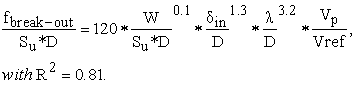
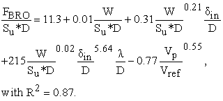
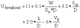
In this study, the horizontal resistance at break-out, F_break-out, is expressed in dimensionless fashion as 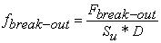. Analysis of more than 75 studies in medium-size and large scale soil tanks showed that f_break-out depends on the current vertical load (W) (here weight of pipe for the whole loading), the normalized initial embedment (δ_in), boundary length (λ) and the rate of axial loading (V_p). It is considered that F_break-out is comprised of a frictional component of resistance below the pipe, installation properties and inherent properties of the pipeline system. The average undrained shear strength calculated for several points in soft soil was used for normalization. The axial resistance formulae are proposed as:

(3)

(4)

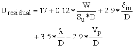
The mobilization of break-out resistance occurs within a pipe movement of less than a half of a diameter, while residual resistance occurs between three to eight times the diameter of the pipe. Horizontal resistance denoted by f_residual=F_residual/S_uD. Classical plasticity solutions for sliding failure of a surface foundation leads to a value of F/W=0.39. However, this value overestimates the resistance for very soft soil range investigated in this study. Based on experimental analysis of more than 45 soil pipe test in full-scale tank, the following equation is suggested:

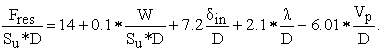(5)

One of the objectives of pipe soil interaction testing was to come up with an empirical model to address axial resistance at every desired point within displacement range, from the onset of movement to breakout resistance and from break resistance to residual steady state resistance. In the following, the main concepts of original p-q model are borrowed to come up with a model that can fully predict the axial frictional behavior of pipe-soil interaction. The modified p-q model, which is called p-q-m, emulates the original model to a certain point call x_f or ε_f (inception of residual trend) and then m parameter deliver the slope of linear interpolation. For better understanding of the p-q-m model, the fundamentals of original p-q model are explained.

A- Original p-q model

Original p-q model was introduced by Vipulanandan and Mebarkia (1990) ^[21] to model the stress-strain relationship of epoxy and polyester polymer concrete behavior in compression. It was presented as:

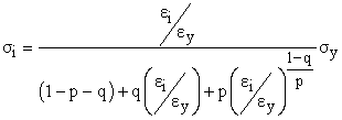(6)

(7)

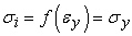
where is the yield strain, the yield strength, the uniaxial stress and uniaxial strain. The parameters p and q are functional variable of the material, different from the known hydrostatic pressure q and deviatoric stress p in constitutive modeling. They are function of the initial modulus E_i and the secant modulus at yield E_sy, which in turn can be defined as:

(8)

(9)

(10)

The model imposed at all time that

(11)

(12)

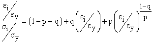
Normalizing the stress by yield stress and the strain by the yield strain,

(13)

(14)

Eq. (7) changes to

(15)

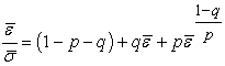
Mantrala and Vipulanandan (1995) ^[22] presented a modified stress-strain model, which provided the following relationship:

(16)

in which q is defined as,

(17)

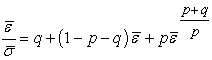
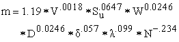
q is, therefore, a direct quantification of the material nonlinear elastic stress-strain behavior , and p is a material property. The normalized stress-strain (or force-displacement) relationships, of the model prediction, are shown in Table 1 for values of q and range of p.

B- p-q-m Model

According to experimental results, force displacement responses of axial tests consist of two stages. Firstly, the force (F) reaches a maximum value which is embodied as y_c (or ) at displacement(u) of x_c (). Secondly, the force declines to the limiting value of residual force presented by y_f . The start of limiting behavior is at displacement of x_f (). In Eq. (18), the symbol represents the floor function and represents absolute value function. In addition, p,q and m parameters are function of rate of loading (V_p) , undrained shear strength (S_u), weight of pipe (W) , pipe diameter (D), initial embedment, boundary length and number of cycles (N). The discrepancy in measured and predicted values for these three parameters (p,q and m) were less than 10 %. The proposed p-q-m model is:

Table 1. Original model normalized stress-strain relationship prediction

Download as

PowerPoint Slide

Larger image(png format)

• Tables index

Veiw figure

View current table in a new window

View next table

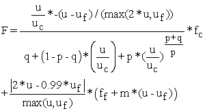(18)

where the parameters are as:

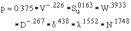(19)

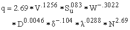(20)

(21)

Break out and residual displacement are

(22)

(23)

In Eq. (18), f_c is equal to f_break-out and f_f is equal to f_residual. These two values are calculated from Eqs. (4) and (5) and u_break-out and u_residual are calculated form Eqs. (22) and (23).

5. Results and Discussions

Download as

• PPT
  PowerPoint Slide
• PNG
  Larger image(png format)

Veiw figureFigures index

•  NEW
  View larger figure in new window
• PREV
  View previous figure

View next figure

Figure 5. Variation of shear strength with water content of soils with (0 kPa < Su < 10 kPa)

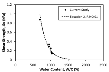
The variation of the soft soil undrained shear strength with the water content for undrained shear strength in the range of 0 kPa to 10 kPa and 0 kPa to 1 kPa are shown in Figure 5 and Figure 6 respectively. Among 92 data points collected from literature, Eq. 1 was used to model the general trend of the decrease of the shear strength as the water content increased, as shown clearly in Figure 5. However, for the soft soil with the high water content (W/C > 500), the second proposed model (Eq. 2) was in a very good agreement with the experimental data having coefficient of correlation (R²) up to 0.91. Since the water content can be quantified directly in the laboratory, this model (Eq. 2) was used to predict the shear strength of the ultra-soft soil in terms of its water content during axial testing of pipe soil interaction.

Download as

• PPT
  PowerPoint Slide
• PNG
  Larger image(png format)

Veiw figureFigures index

•  NEW
  View larger figure in new window
• PREV
  View previous figure

View next figure

Figure 6. Variation of shear strength with water content of soils with (0 kPa < Su < 1 kPa).

Download as

• PPT
  PowerPoint Slide
• PNG
  Larger image(png format)

Veiw figureFigures index

•  NEW
  View larger figure in new window
• PREV
  View previous figure

View next figure

Figure 7. Comparison of the measured and predicted breakout resistance calculated from Eq. 3.

Download as

• PPT
  PowerPoint Slide
• PNG
  Larger image(png format)

Veiw figureFigures index

•  NEW
  View larger figure in new window
• PREV
  View previous figure

View next figure

Figure 8. Comparison of the measured and predicted breakout resistance from different projects [23]

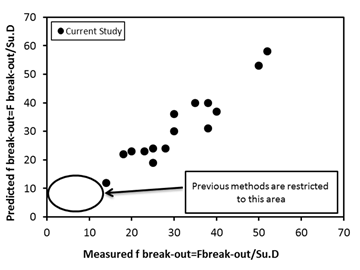
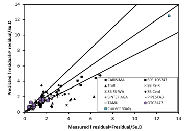
The relationship between the measured and predicted normalized breakout resistance is shown in Figure 7. It is obvious that the previous methods are restricted to normalized breakout resistance with values less than 10. However, the experimental normalized breakout resistances that are greater than 10 were predicted very well by using the new provided model (Eq. 3). In addition, the new model (Eq.3) is used to predict a set of data from literature as shown in Figure 8 ^[20]. The reported data of f_break-out resistance were predicted very well using Eq. (3).

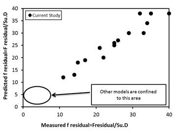
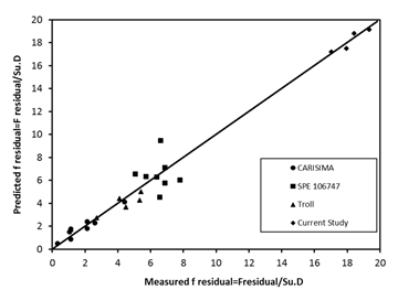
The relationship between the measured and predicted normalized residual resistance is shown in Figure 9. It is clearly indicated that the previous methods are restricted to normalized residual resistance with values less than 10. However, the experimental normalized residual resistances that are greater than 10 were predicted very well using the new provided model (Eq. 5). The new model (Eq.5) is used to predict a set of data from literature as shown in Figure 10 ^[20]. The reported data of f_residual resistance were predicted very well using Eq. (5) and most of these were estimated perfectly.

Download as

• PPT
  PowerPoint Slide
• PNG
  Larger image(png format)

Veiw figureFigures index

•  NEW
  View larger figure in new window
• PREV
  View previous figure

View next figure

Figure 9. Comparison of the measured and predicted residual resistance calculated from Eq. 3.

Download as

• PPT
  PowerPoint Slide
• PNG
  Larger image(png format)

Veiw figureFigures index

•  NEW
  View larger figure in new window
• PREV
  View previous figure

View next figure

Figure 10. Comparison of the measured and predicted residual resistance from different projects.

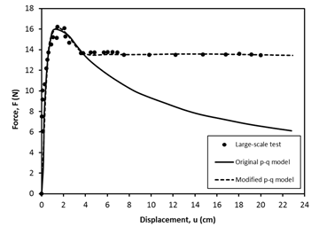
The new developed model (p-q-m) is used to predict the full range behavior of force-displacement relationship of axial pipe-soil interaction in soft soil as shown in Figure 11. A comparison between the original and new p-q is identified where the original p-q model failed to predict the force values beyond the peak and the model diminished quickly. However, the new p-q model was able to predict the force values before and after the peak with very good agreement with the experimental values.

Download as

• PPT
  PowerPoint Slide
• PNG
  Larger image(png format)

Veiw figureFigures index

•  NEW
  View larger figure in new window
• PREV
  View previous figure

Figure 11. Test results are characterized by p-q and p-q-m model

A statistical analysis has been performed on the full force-displacement model for axial pipe soil interaction using four different strategies as follows ^[24]:

1. Regression Analysis.

2. Error Estimation Analysis.

3. Classical Statistical Method.

4. Cumulative Probability Function.

In each of the above methods, the accuracy of model prediction has been evaluated and the best ranking was given to the more accurate one; then followed by the overall ranking procedure, which summed up all the ranking numbers for each one from every single method and the lowest accumulative number was ranked as the best one.

Based on the results shown in Table 1, it is necessary to have more than one statistical method for best data modeling procedure. Through overall ranking procedure, the real and accurate data modeling can be established since it is an accumulative result of several applied statistical methods. It is clearly shown that the modified p-q model had better estimation than the original p-q model throughout all applied statistical methods. As a result, the overall evaluation ranks the modified p-q as the best model and the original p-q model to be the worst in modeling axial pipe soil interaction.

Table 1. Summary of Statistical Analysis of p-q and m-p-q Models

Download as

PowerPoint Slide

Larger image(png format)

• Tables index

Veiw figure

View current table in a new window

View previous table

6. Conclusions

Based on the results of this study, the following conclusions can be advanced:

1. Large-scale model test was experimentally instrumented and tested to represent the real behavior of pipe-soil interaction on ultra-soft soil condition.

2. A new innovated Remote Gridding System (RGS) was developed to capture soil surface displacement field and berm formation at vicinity of pipe.

3. Two new models were used to correlate the shear strength with the water content of the ultra-soft soil. The first model was verified with a set of 92 data points reported in the literature. While the second model was verified with experimental tests on ultra-soft soil with high water content. The second model strongly correlated the shear strength with water content of ultra-soft soil with coefficient of correlation (R²) up to 0.91. Hence, this model (Eq.2) had practical benefit to be used to quantify the shear strength of ultra-soft soil in terms of its water content.

4. New analytical models were developed to predict the axial break-out resistance and large-displacement residual resistance for pipe-soil interaction in ultra-soft soil. The new models were functions of several parameters such as vertical loads (W), normalized initial embedment (δ_in), boundary length (λ), and the rate of axial loading (V_p). The new models were verified with experimental results and their predictions were very good with coefficient of correlation (R²) up to 0.87.

5. To model the full force-displacement behavior of axial testing of pipe in ultra-soft soil, a new analytical model (p-q-m) was proposed. The new proposed model was developed using the basis of original p-q model after making necessary modifications. The new model (p-q-m) showed a very good agreement with the experimental testing results of force-displacement relationship of axial pipe-soil interaction. However, the original p-q model failed to predict the force values beyond the peak and the model diminished quickly.

6. Extensive statistical procedure has been used to analyze the performance of both p-q and m-p-q models in modeling full range force-displacement relationship for axial pipe soil interaction in ultra-soft soil. It has been shown that the m-p-q model had the best estimation using any of the statistical methods.

Acknowledgement

This study was supported by the Center for Innovative Grouting Materials and Technology (CIGMAT), University of Houston, Houston, Texas. The help and support of professor Vipulanandan is greatly appreciated.

References

[1]	Guo B., Son S., Chacko J., and Ghalambor A. (2005). “Off-shore Pipelines,” Elsevier Inc.
	In article
[2]	Champiri, M. D., Mousavizadegan, S. H., Moodi, F. (2012). “A Decision support system for diagnosis of distress cause and repair in marine concrete structures,” International journal of Computers and Concrete, Techno press, Vol. 9, No. 2, pp. 99-118.
	In article
[3]	Champiri, M. D., Mousavizadegan, S. H., Moodi, F. (2012). “A fuzzy classification system for evaluating health condition of marine concrete structures,” Journal of Advanced Concrete Technology, Vol. 10, pp. 95-109.
	In article		View Article
[4]	Bruton D., Carr M., White D. J., and Cheuk J. C. Y. (2008). “Pipe-Soil Interaction During Lateral Buckling and Pipeline Walking,” The SAFEBUCK JIP.
	In article
[5]	Bai Y. and Bai Q. (2005). “Subsea Pipelines and Risers,” Elsevier Ltd.
	In article
[6]	Foss P. (2013). “Guidance”, Spring of 2013.
	In article
[7]	Dixon D.A. and Rultledge D.R. (1968). “Stiffened Catenary Calculation in Pipeline Laying Problem.,” J Eng Ind; Vol.(90B), No.(1), pp.153–60.
	In article		View Article
[8]	Lenci S. and Callegari M. (2005). “Simple Analytical Models for the J-Lay Problem,” Acta Mech , Vol.(178), pp.23-39.
	In article
[9]	Chai Y.T. and Varyani K.S. (2006). “An Absolute Coordinate Formulation for Three- Dimensional Flexible Pipe Analysis,” Ocean Eng., Vol.(33), pp.23-58.
	In article
[10]	Wang D., White D. J. and Randolph M. F. (2010). “Large-Deformation Finite Element Analysis of Pipe Penetration and Large-Amplitude Lateral Displacement,” Can. Geotechnical J., Vol. (47), No.(8), pp. 842-856.
	In article
[11]	Lyons C.G. (1973). “Soil Resistance to Marine Lateral Sliding Pipe Lines,” Dallas (TX), OTC.
	In article
[12]	Wantland G.M., O'Neill M.W., Reese L.C. and Kalajian E.H. (1979). “Lateral Stability of Pipelines in Clay,” Houston, USA, OTC-3477-MS.
	In article
[13]	Lambrakos K.F. (1985). “Marine Pipeline Soil Friction Coefficients from In-Situ Testing,” Ocean Engineering, Vol.(12), No.(2), pp.131-50.
	In article
[14]	Brennodden H., Sveggen O., Wagner D.A.and Murff J.D. (1986). “Full-Scale Pipe-Soil Interaction Tests,” Houston, USA, OTC 5338-MS.
	In article
[15]	Murff J.D., Wagner D.A. and Randolph M.F. (1989). “Pipe Penetration in Cohesive Soil,” Geotechnique, Vol.(39), No.(2), pp.213-229.
	In article
[16]	Joshaghani, M.S ., Raheem A.M. (2014) “ Full-scale Testing and Numerical Modeling of Axial and Lateral Soil Pipe Interaction in Deepwater” Recent Advances in Continuum-Scale Modeling of Flow and Reactive Transport in Porous Media Posters , 2014 AGU Fall Meeting.
	In article		PubMed
[17]	Mebarkia S. (2006). "Effect of High-Pressure/High-Temperature Flowlines and Soil Interaction on Subsea Development,” Houston, USA, OTC 18107-MS.
	In article
[18]	Vipulanandan, C., Yanhouide, J. A., & Joshaghani, S. M. (2013). “Deepwater Axial and Lateral Sliding Pipe-Soil Interaction Model Study,” Pipelines 2013, Pipelines and Trenchless Construction and Renewals-A Global Perspective, ASCE, pp. 1583-1592.
	In article		View Article
[19]	Raheem, A. M., and Joshaghani, M. S. (2016). “Modeling of Shear Strength-Water Content Relationship of Ultra-Soft Clayey soil,” International Journal of Advanced Research (2016), Volume 4, Issue 4, pp. 537-545.
	In article		View Article
[20]	Raheem A.M., Vipulanandan C. and Ayoub A. (2013). “Shear Strength Relationship for Very Soft Clayey Soils,” Proceeding of CIGMAT Conference & Exhibition, Houston, USA.
	In article
[21]	Vipulanandan C. and Mebarkia S. (1990). “Effect of Strain Rate and Temperature on the Performance of Epoxy Mortar,” Polymer Engineering and Science, Vol. 30, No. 2, pp. 734-740.
	In article		View Article
[22]	Mantrala, K S , Vipulanandan, C. (1995). “Nondestructive Evaluation of Polyester Polymer Concrete,” ACI Materials Journal, Vol. 92, No. 6, pp. 660–68.
	In article
[23]	Bruton D., White D., Cheuk C., Bolton M., and Carr M. (2006). “Pipe/Soil Interaction Behavior During Lateral Buckling,” SPE Projects, Facilities & Construction, pp. 1-9.
	In article		View Article
[24]	El-Sakhawy N.R., Youssef K. M. and Badawy R. A. E. (2008),”Prediction of the Axial Bearing Capacity of Piles by Five-Cone Penetration Test Based Design Methods”, (IAMAG),1-6 Oct 2008,India.
	In article