The paper investigates the comparative effects of several random sampling methods on the maximum likelihood estimates of a simple logistic regression model. The study uses simulated data (logistic populations with pre-defined parameter values) that used Monte Carlo methods to simulate. Sampling techniques include Simple Random Sampling (SRS) and six variations of Stratified Sampling where two are single-stage Stratified Sampling and four are choice-based (two-phase) Stratified Sampling. Parameter estimates arising under each sampling technique were compared using performance measures Bias, Standard Error & Percentage of models that are feasibly estimated. The simulation-based analysis found that choice-based sampling with proportional allocation in both phases is the best-suited sampling technique for parameter estimation of a simple logistic regression model.
The sample size and technique to use when fitting a logistic model are important areas of concern. Studies have shown that maximum likelihood estimates (MLEs) are biased when the sample size is too small 1. Also, it has been identified that parameter estimates of logit and probit models are unstable (high variation) for small samples 2. Hence, studies have been conducted to find a suitable sample size for a logistic model. The paper 3 gives a formula for calculating the sample size for logistic regression with a small response probability and found that the required sample size is very sensitive to the distribution of predictors. Hence, diverse methods yield different sample sizes depending on the distribution of predictors. Using the formula in 3, paper 4 gives a sample size table for logistic models. The table assumes that predictors are continuous and have a joint multivariate normal distribution, and this table is best suited for models with one covariate. These studies have focused solely on the effect of sample size, but it is also important to study the rate of improvement of parameter estimates with sample size and the effect of sampling techniques on the bias and precision of parameter estimates.
The studies 5, 6, 7 look into parameter estimates of the logistic model arising from various sampling strategies. These studies show that sample size and sampling strategy both affect the small sample bias of the maximum likelihood estimator and the precision of the subsequent estimates. All these studies use real-world data-sets 5 or data simulated according to real-world situations 6, 7 in the experiments. However, none of these analyze the behavior of sampling techniques with different characteristics of the logistic populations (odds ratio, population proportion). Therefore, a more comprehensive look into this area is essential.
This study uses Monte Carlo simulation methods to simulate multiple population data. Populations were generated according to predefined parameter values, and repeated samples from these populations were taken using various random sampling techniques. The sampling techniques used include simple random sampling and six variations of stratified sampling. Samples with different sample sizes were taken from each population using these sampling techniques, and logistic models were fitted for these samples. Parameter estimates arising under each sampling technique were studied with odds ratio, population proportion of success and sample size using the performance measures “bias,” “standard error,” and “percentage of models that are feasibly estimated.”
The remainder of this article is structured as follows. Section 2 provides details regarding the theories and methodologies that were used in the study. The data simulation and sampling approaches are discussed in Section 3. Section 4 provides details regarding the testing procedures and findings of the study. The major findings and limitations of the study are provided in Section 5.
This study uses random sampling techniques in which every unit in the population has some chance of being selected for a sample. Further, sampling without replacement was used for all of the sampling techniques. The first sampling technique is simple random sampling, the easiest to understand and apply. The other sampling strategies used are variations of stratified random sampling. Both independent and dependent variables were used for stratification. We used both equal and proportional allocation methods. In equal allocation, equal numbers of units from each stratum are selected to fill the sample, and in proportional allocation, the number of units from each stratum selected for the sample is proportional to the size of the stratum. Six variations of stratified sampling were used in the study, two with single-stage stratified sampling and four with choice-based (two-stage) stratified sampling.
In single-stage stratified sampling, stratification is performed using only independent variable:
• Stratify based only on independent variable using equal allocation.
• Stratify based only on independent variable using proportional allocation.
Choice-based stratified sampling involves two stages of sampling. In the first stage, the number of cases required from each category of response is determined. Samples are taken according to the number of cases. In the second phase, a stratified sample is taken from the previous sample with the stratification variable being the independent variable:
• Use equal allocation in both the first and the second stages.
• Use equal allocation in the first stage and proportional allocation in the second.
• Use proportional allocation in the first stage and equal allocation in the second.
• Use proportional allocation in both the first and the second stages.
2.2. Maximum Likelihood Estimation of a Logistic Regression ModelIn contrast to linear regression, logistic regression has no closed-form expression for the coefficient values that maximize the likelihood function. Therefore, an iterative process such as the Newton-Raphson method is used. Such a process begins with an initial guess and then revises it until it converges to a specific value. In some instances, the MLE does not converge. This indicates that the parameter estimates are not meaningful, because the iterative process was unable to find appropriate solutions. Failure to converge can occur for several reasons;
• Having too many independent variables and too few observations (cases) 8.
• Multicollinearity between predictor variables 9.
• Separation (complete or quasi-complete) in the sample 10.
This study only considers separation, as other kinds of situations are not encountered.
Complete separation in logistic regression occurs when a linear combination of the predictors yields a perfect prediction of the response variable. As an example, consider the sample in Table 1, in which Y is the response variable and X is the predictor variable.
From the example, it is clear that if X ≥ 4, then Y = 1, and if X < 4 then Y = 0. This is an example of complete separation.
According to 10, if a sample is completely separated, then the MLEs are not unique and do not converge
Similar to complete separation, quasi-complete separation in logistic regression occurs when the outcome variable separates a predictor variable or a combination of predictor variables to some degree. As an example, consider the sample in Table 2, in which Y is the response variable and X is the predictor variable.
In the above sample, if X < 4, then Y = 0, and if X > 4 then Y = 1, but if X = 4 then Y could be zero or one. This overlap in the middle range of the data renders the separation quasi-complete. It is highly unlikely that quasi-complete separation will occur with truly continuous data. Therefore, this situation will not be encountered in the study, as the study used a continuous independent variable. Again, in this instance, the MLEs of the model coefficients are not unique and do not converge 10.
If complete or quasi-complete separation does not occur in the sample, then there is an overlap in the sample points. In this situation, the MLEs exist and are unique 10.
2.3. Fitting a Logistic Regression Model Using R SoftwareThis study was conducted using the statistical software R to fit logistic models to the derived samples. For some samples, warning messages occurred during the fitting of the logistic model.
1. glm.fit: Algorithm Did Not Converge
The “stats” package in R estimates parameters of a logistic regression model using the maximum likelihood method, which uses the iterative Newton-Raphson method. In this process, an initial value for a parameter estimate is guessed, and this value is then revised until the value converges to a specific value. If the value does not converge after a specified number of iterations (this number can be changed), then R returns the last iteration value as the parameter estimate with a warning message to that effect.
2. glm.fit: Fitted Probabilities Numerically Zero or One Occurred
Consider the simple logistic model ln (P/1−P) = β0 + β1·X. Here, a logistic regression model is used to calculate the probability of success P for a given X value. Since the ratio P/1−P doesn’t exist for P = 1 and P = 0, P must be in the interval (0, 1) for all values of X in the logistic model. Therefore, in a fitted model, if the estimated probability of success is zero or one for some (or all) X values, then R returns a warning message to that effect with the parameter estimates of the fitted model.
2.4. Performance Measures for Comparing Sampling TechniquesBias = |E( ) − β| and Standard Error = standard deviation of the sampling distribution of
  where β is the parameter,
  is the MLE of β and E(
 ) is the expected value of
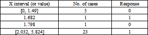
For some samples, during the fitting of a logistic model using R, both of the above warnings occur, and for some samples, only the second occurs. It was found from the examination of these samples that if both warnings occur, the sample is completely separated, and if only the second warning occurs, the sample is not separated, but for a large range of X values, the response is only one or zero. As an example, consider the sample in Table 3.
The X interval [2.03, 5.82] yields only the value one. Therefore, models fitted for this kind of sample will yield a fitted probability that is extremely close to one (e.g., values such as 0.9999999999) for X values around 5.824. In these instances, R cannot distinguish these fitted probability values from one and considers the model as a perfect fit (i.e., P(X = 5.824) = 1). Theoretically, this cannot happen in a logistic model, because when P equals one, P/1−P goes to infinity, thereby generating a warning message. However, this sample has an overlap. Therefore, the MLEs of the logistic model do converge to a unique value. This study requires models that have unique estimates. Hence, models that result in both of the discussed warnings were considered as models that are not feasibly estimated.
Models fitted to samples with complete separation are quite good at classifying observations, but inferences regarding population parameters from those models are to be avoided, because the coefficients of those models are large. Therefore, during the calculation of the other two performance measures, estimates of samples where both warnings occur were omitted.
Because simple logistic regression was considered in this study, only one independent variable was considered when simulating population data. Populations of size 100,000 were generated according to the simple logistic regression model, ln (P/1−P) = β0 + β1·X. Here, the independent variable (X) is considered to follow a normal distribution. Since normal distributions can be used to model a wide range of real-world data, the use of a normal distribution as the distribution of the independent variable will enable the simulated population to reflect qualities of a real-world logistic population.
Values for the parameter β1 were pre-decided according to the required odds ratio, and the range for the independent variable was derived by manipulating the mean and standard deviation. To obtain the required population proportion of success (PS), each population was generated using trial and error, where the value of β0 was changed until the required proportion was achieved. Since it is difficult to achieve an exact PS, the required proportions were defined as ranges. The ranges were 0.08-0.12, 0.23-0.27, and 0.48-0.52. The reason for generating populations with different population proportions of success is to study the effect of the PS on the logistic regression model. Here, a high PS (PS greater than 0.6) was not considered. A population with a high PS will simply interchange the numbers of zeroes and ones of a population with a low PS. For example, consider two populations with the proportions of success of 0.2 and 0.8. The first population’s responses will consist of 20,000 ones and 80,000 zeroes, and the second population’s responses will consist of 20,000 zeroes and 80,000 ones. Therefore, low proportions of success will have the same effect on a logistic model as high proportions of success.
The algorithm below specifies how Population 1 was generated (refer to Table 4 for the parameter values of Population 1).
3.1. Algorithm for Generating Population 1• Generate 100,000 random numbers from a normal distribution with a mean of six and a standard deviation of one. Let these numbers be denoted by X.
• Designate an arbitrary value for β0 (use a pre-decided value for β1).
• Calculate P values corresponding to each X value using P = 1/(1 + exp(β0 + β1·X)).
• Generate 100,000 random numbers from a Bernoulli distribution using the P values calculated above. Let these generated numbers be denoted by Y. Here, the generated numbers will include only zeroes and ones (Y is binary).
• Calculate the PS: PS = ∑Y/100,000.
• If PS is in the range 0.08-0.12, we consider the generated X and Y values as our population. Otherwise, go to step 2 and repeat this procedure until PS is in the range of 0.08-0.12.
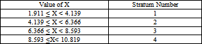
For this study, it was considered that there are four strata for both ranges of populations. This is a subjective number, as another person could decide on different numbers of strata. However, considering too few strata will result in high within-strata variation. Moreover, the number of strata can be increased only up to a specific level, as the inclusion of too many strata will reduce the practicality and increase the complexity of the stratified sampling procedure. Therefore, considering the above facts and the researchers’ convenience, the number of strata was designated as four. Table 5 and Table 6 show how the stratification variable was created.
Sample sizes of 30, 60, 90, 150, 210, and 300 were considered for this study. For each sample size and population combination, 1,000 samples were taken using each sampling technique. For example, 1,000 samples of size 30 were taken from Population 1 using simple random sampling. This procedure was repeated for all of the other sampling techniques as well. Samples were also drawn in this manner using the seven sampling techniques for all of the other combinations.
MLEs typically perform well with respect to three performance measures for large samples. However, since taking large samples is not practical most of the time, estimates from small samples (size 30) must be analyzed extensively.
Note. The following denotations will be included in figures. SRS: simple random sampling; STR-Equal: stratified sampling with equal allocation; STR-Prop: stratified sampling with proportional allocation; Equal-Equal: choice-based sampling with equal allocation from choice and covariate; Equal-Prop: choice-based sampling with equal allocation from choice and proportional allocation from covariate; Prop-Equal: choice-based sampling with proportional allocation from choice and equal allocation from covariate; Prop-Prop: choice-based sampling with proportional allocation from choice and covariate.
4.1. Comparison of Sampling Techniques with Odds RatioFigure 1, Figure 2 and Figure 3 compare how the sampling techniques perform for various odds ratios when the PS is approximately 0.1, the sample size is 30, and the range of X is 1.911-10.819.

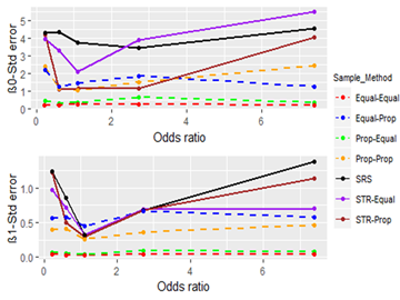

From Figure 1, it is clear that the choice-based sampling techniques other than Prop-Prop sampling yield biased estimates for both parameters. One-stage sampling and Prop-Prop sampling yield less biased estimates and perform virtually the same with respect to bias measurement. Another fact visible from it is that the estimates of β1 are less biased than the estimates of β0 for all of the sampling techniques. According to Figure 2, choice-based samples yield estimates with low standard error than that of one-stage samples. Among the choice-based samples, the standard error values of the Equal-Equal and Prop-Equal sample estimates are extremely low. Also, the estimates for β1 have lower standard errors than the estimates for β0 for all sampling techniques. Figure 3 indicates that choice-based sampling outperforms one-stage sampling with respect to the percentage of feasible models. When we compare the performances of one-stage sampling techniques with respect to the feasible model percentage, we see that there is no noteworthy difference among the three sampling techniques and that this is also the case for the four choice-based sampling techniques.
When we consider all three performance measurements, the estimates usually perform well when the odds ratio is approximately one for all of the sampling techniques. From the figures, it seems that when the odds ratio is not equal to one, the estimates are more prone to underperform for all sampling techniques. Further, when the odds ratio is either low or high, the estimation behavior does not vary in a major manner. Consider, for example, the bias values derived when the odds ratios are 0.223 and 7.389. The bias values for a particular sampling technique in these instances are very similar.
4.2. Comparison of Sampling Techniques with Proportions of SuccessFigure 4, Figure 5 and Figure 6 compare how the sampling techniques perform for various proportions of success, when the odds ratio is 0.223, the sample size is 30, and the range of X is 1.911-10.819.
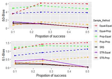
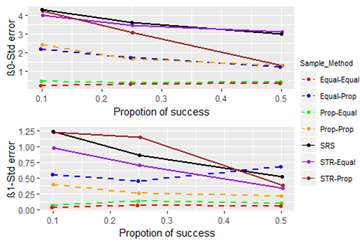
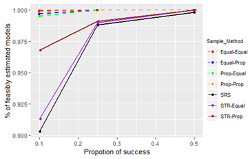
In this instance also, the behavior of the sampling techniques is similar as before (high bias in choice-based and high standard error in single staged). When consider all three performance measurements, we can see that estimates perform comparatively well when the PS is approximately 0.5, i.e. bias, standard error is low and feasible percentage high when PS is around 0.5 for all sampling techniques.
Further, by considering the analysis in the above sections, we can infer that the performance of a sampling technique does not depend on the odds ratio or PS. That is, if one sampling technique performs better than another, this would not change significantly when the odds ratio or PS changes.
4.3. Comparison of Sampling Techniques with Sample SizesThe previous analysis showed that estimates are more prone to underperform when the odds ratios are very low (or very high) or the proportions of success are very low (or very high). Hence, it is necessary to identify the sampling techniques that perform well in situations that might yield problematic estimates. Therefore, the best populations for comparing sampling techniques properly are Populations 1 and 8.
Previous studies have shown that the sample size plays a vital role in deriving estimates that are unbiased and precise 1, 2. Figure 7, Figure 8 and Figure 9 compare the estimates derived using each sampling technique with the sample sizes in Population 1 (the range of X is 1.911-10.819).
In this situation also, choice-based techniques perform better than one-stage techniques with respect to the standard error and feasible model percentage. With respect to bias, one-stage techniques perform better than choice-based techniques except for Prop-Prop sampling. Further, it is clear that all of the sampling techniques perform increasingly well with increasing sample size.

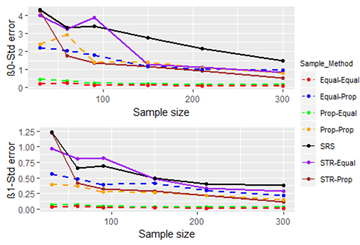
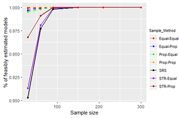
Figure 10, Figure 11 and Figure 12 give the performance of sampling techniques with the sample size for Population 8 (range of X is 9.110-98.190).
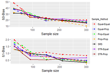
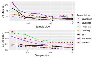
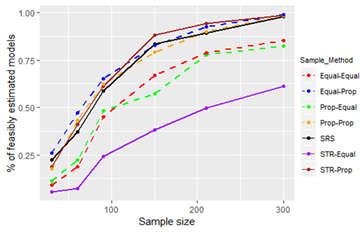
Figure 10 - Figure 11 show that the bias and standard error of the estimates from all of the sampling techniques do not differ greatly. However, when we consider the percentage of feasible models, there is a clear difference between the sampling techniques. The sampling techniques that use a proportional allocation from the independent variable (X) together with SRS outperform the other sampling techniques. Sampling technique STR-Equal is the most underperforming sampling technique, whereas sampling techniques Prop-Equal and Equal-Equal perform better than STR-Equal.
When we compare the performance measures of the sample estimates from Populations 1 and 8, we see that there is a visible difference. This difference is highly visible in estimates derived for β0 as the bias, and the standard error values are very high in population 8. On the whole, sampling techniques perform poorly with respect to bias and standard error even for the relatively large sample sizes in Population 8. This indicates that the range of X has a strong impact on sample estimates.
Based on the analysis, it was evident that choice-based sampling with proportional allocation in both phases is the best-suited sampling technique for parameter estimation of a simple logistic regression model. Further, when the range of X is not large, one-stage sampling is recommended over choice-based sampling. Except for both phase proportional allocations, other choice-based sampling techniques tend to yield biased estimates for small samples even though the standard errors of these estimates are comparatively low against one-stage sampling estimates. Further, the use of a choice-based sampling technique will complicate the sampling procedure; therefore, it is always better to use the one-stage sampling technique in such instances because there is no special advantage of using the two-stage sampling technique. In addition, when the range of X is large, an equal allocation is not recommended, as it will have a low chance of obtaining a feasibly estimated model. Furthermore, as the sample size increases, the chance of obtaining a model with high performing estimates increases irrespective of the sampling technique. Moreover, also irrespective of the sampling technique, it is suitable to take a large sample, if any of the following holds:
• The odds ratio is very small or very large.
• The population proportion is very large or very small.
• The range of X is large.
Since the study was based on simulations, some limitations can be identified as follows:
• The generated data were not naturally generated in separate strata. All of the data were generated randomly and assigned into strata defined later.
• Only one independent variable was considered, and it was assumed to be normally distributed. This might not be the case in some practical situations.
• Sampling procedures of stratified sampling in the study are very subjective, especially the number of strata.
In addition to the above, we do not adjust for sampling design where the sampling weights are used in the estimation of models. Future studies in this topic can further investigate this area by incorporating estimators that are adjusted for sampling design in the study.
| [1] | Amemiya, T., “The n-2-Order Mean Squared Errors of the Maximum Likelihood and the Minimum Logit Chi-Square Estimator”, The Annals of Statistics, 8 (3), 488-505, 1980. | ||
| In article | View Article | ||
| [2] | Gordon, D.V., Lin, Z., Osberg, L. and Phipps, S., “Predicting Probabilities: Inherent and Sampling Variability in the Estimation of Discrete-Choice Models”, Oxford Bulletin of Economics and Statistics, 56 (1), 13-31, 1994. | ||
| In article | View Article | ||
| [3] | Whittemore, A.S., “Sample Size for Logistic Regression with Small Response Probability”, Journal of the American Statistical Association, 76 (373), 27-32, 1981. | ||
| In article | View Article | ||
| [4] | Hsieh, F.Y., “Sample size tables for logistic regression”, Statistics in medicine, 8 (7), 795-802, 1989. | ||
| In article | View Article PubMed | ||
| [5] | Breslow, N. E., and Chatterjee, N., “Design and analysis of two‐phase studies with binary outcome applied to Wilms tumour prognosis”, Journal of the Royal Statistical Society: Series C (Applied Statistics), 48 (4), 457-468, 1999. | ||
| In article | View Article | ||
| [6] | Giles, J. A., and Courchane, M. J., “Stratified sample design for fair lending binary logit models”, Department of Economics, University of Victoria, 2000. | ||
| In article | |||
| [7] | Dietrich, J., “The effects of sampling strategies on the small sample properties of the logit estimator”, Journal of Applied Statistics, 32 (6), 543-554, 2005. | ||
| In article | View Article | ||
| [8] | Peduzzi, P., Concato, J., Kemper, E., Holford, T. R., and Feinstein, A. R., “A simulation study of the number of events per variable in logistic regression analysis”, Journal of clinical epidemiology, 49 (12), 1373-1379, 1996. | ||
| In article | View Article | ||
| [9] | Schaefer, R. L., “Alternative estimators in logistic regression when the data are collinear”, Journal of Statistical Computation and Simulation, 25 (1-2), 75-91, 1986. | ||
| In article | View Article | ||
| [10] | Albert, A. and Anderson, J.A., “On the existence of maximum likelihood estimates in logistic regression models”, Biometrika, 71 (1), 1-10, 1984. | ||
| In article | View Article | ||
Published with license by Science and Education Publishing, Copyright © 2021 Oshada Senaweera, Prasanna S. Haddela and Gayan Dharmarathne
![]() This work is licensed under a Creative Commons Attribution 4.0 International License. To view a copy of this license, visit
http://creativecommons.org/licenses/by/4.0/
This work is licensed under a Creative Commons Attribution 4.0 International License. To view a copy of this license, visit
http://creativecommons.org/licenses/by/4.0/
| [1] | Amemiya, T., “The n-2-Order Mean Squared Errors of the Maximum Likelihood and the Minimum Logit Chi-Square Estimator”, The Annals of Statistics, 8 (3), 488-505, 1980. | ||
| In article | View Article | ||
| [2] | Gordon, D.V., Lin, Z., Osberg, L. and Phipps, S., “Predicting Probabilities: Inherent and Sampling Variability in the Estimation of Discrete-Choice Models”, Oxford Bulletin of Economics and Statistics, 56 (1), 13-31, 1994. | ||
| In article | View Article | ||
| [3] | Whittemore, A.S., “Sample Size for Logistic Regression with Small Response Probability”, Journal of the American Statistical Association, 76 (373), 27-32, 1981. | ||
| In article | View Article | ||
| [4] | Hsieh, F.Y., “Sample size tables for logistic regression”, Statistics in medicine, 8 (7), 795-802, 1989. | ||
| In article | View Article PubMed | ||
| [5] | Breslow, N. E., and Chatterjee, N., “Design and analysis of two‐phase studies with binary outcome applied to Wilms tumour prognosis”, Journal of the Royal Statistical Society: Series C (Applied Statistics), 48 (4), 457-468, 1999. | ||
| In article | View Article | ||
| [6] | Giles, J. A., and Courchane, M. J., “Stratified sample design for fair lending binary logit models”, Department of Economics, University of Victoria, 2000. | ||
| In article | |||
| [7] | Dietrich, J., “The effects of sampling strategies on the small sample properties of the logit estimator”, Journal of Applied Statistics, 32 (6), 543-554, 2005. | ||
| In article | View Article | ||
| [8] | Peduzzi, P., Concato, J., Kemper, E., Holford, T. R., and Feinstein, A. R., “A simulation study of the number of events per variable in logistic regression analysis”, Journal of clinical epidemiology, 49 (12), 1373-1379, 1996. | ||
| In article | View Article | ||
| [9] | Schaefer, R. L., “Alternative estimators in logistic regression when the data are collinear”, Journal of Statistical Computation and Simulation, 25 (1-2), 75-91, 1986. | ||
| In article | View Article | ||
| [10] | Albert, A. and Anderson, J.A., “On the existence of maximum likelihood estimates in logistic regression models”, Biometrika, 71 (1), 1-10, 1984. | ||
| In article | View Article | ||


