Premium pricing is always a challenging task in general insurance. Furthermore, frequency of the insurance claims plays a major role in the pricing of the premiums. Severity in insurance on the other hand, can either be the amount paid due to a loss or the size of the loss event. For insurer’s to be in a position to settle claims that occur from existing portfolios of policies in future, it is necessary that they adequately model past and current data on claim experience then use the models to project the expected future experience in claim amounts. In addition, non-life insurance companies are faced with problems when modeling claim data i.e selecting appropriate statistical distribution and establishing how well it fits the claimed data. Therefore, the study presents a framework for choosing the most suitable probability distribution and fitting it to the past motor claims data and the parameters are estimated using maximum likelihood method (MLE). The goodness of fit of frequency distributions was checked using the chi-square test and Anderson-Darling tests was applied to severity claim distributions. Best chosen models from frequency models and severity models were used to estimate the expected claim amount per risk in the following year. The study employed AIC to choose between competing models. Pareto and Negative Binomial model best fit severity claims, and frequency claims respectively. The two models were used for projection.
In the classical Bonus-Malus System (), the transition rule is governed by frequency; it ignores the severity information, which implies that the future loss of a policyholder can be appropriately modeled by predicting the frequency only, 1 and 2. In reality, this frequency-driven transition rule is the standard practice in many jurisdictions. It carries an implicit assumption that the frequency and severity are independent, such that the premium can be simply computed as a product of the mean frequency and mean severity. Theoretically, the structure of the traditional is directly related to the classical theory of the collective risk model, which assumes independence between frequency and severity for mathematical tractability and convenience, 3. However, a series of recent empirical studies have shown that the dependence between frequency and severity in auto insurance is statistically significant 4, 5. This phenomenon invalidates the practice of using frequency-driven and highlights the need to extend the classical collective risk model by allowing some dependence structure between frequency and severity. Existing studies on dependent frequency-severity models and the associated insurance premiums include copula-based models 4, 6, two-step frequency-severity models 5, 7, 8, 9, and bivariate random effect-based models 10, 11, 12. The random effect model is especially popular in insurance ratemaking because of the mathematical tractability in its prediction. The bivariate random effect model consists of two random effect components. The first random effect induces the dependence among frequencies and the second induces the dependence among individual severities. These two random effects are then jointly modeled to induce the dependence between frequency and severities at the distribution level. Statistical methods for prediction using the random effect model are well developed in the statistical and insurance literature, such as in; 10, 11, 12. Statistical modeling and analysis for accommodating the various dependent structures in the collective risk models have been actively conducted. For the above reasons, modeling frequency and severity of insurance claims are being done simultaneously globally.
13, did a comparison of risk classification methods for claims severity. They compared several risk classification methods for claim severity data by using weighted equation which was written as a weighted difference between the observed and fitted values. The weighted equation was applied to estimate claim severities which was equivalent to the total claim cost divided by the number of claims. From their data, they also observed that, the classical and regression fitting procedures gave equal values for parameter estimates however, the regression procedure provided a faster convergence. The multiplicative and additive models gave similar parameter estimates. The smallest chi-squares were given by the minimum chi-squares model except for the exponential model. All models provided similar values for absolute difference. This study therefore was meant to come up with best model among the chosen.
2.2. Review of Previous Studies on Insurance Claim FrequencyThe Poisson regression model which is a GLM model was introduced by 14 and deeply looked into by 15. 16 Did put forward the Poisson distribution as the model to be used in modeling frequency of claims. Although it’s statistically conducive and favorable, it emphasized that the Poisson distribution had some shortcomings which limited its usage. The Poisson model had equidispersion property which is the equality of mean and variance. This study has considered wide range of models to come up with best model that can be used in insurance analysis of frequency claims.
Research used secondary data from APA insurance company, from January 2017 to July 2019, regarding motor insurance.
Three assumptions were made on the data before use, these included:
i. All the claims came from the same distribution
ii. Zero claims are assumed to be non-inflated
iii. There exists no catastrophic claim
3.2. Procedures for Processing DataThis section describes the steps that were followed in fitting a statistical distribution to the claim data. There are basic standards that were followed in fitting the various probability distributions under consideration.
These steps were:
i. Choosing the model of distribution.
ii. Estimating probability distribution model parameters.
iii. Check goodness of fit of the model
iv. Specification of the criteria to choose best model from the selected distributions
3.3. Choosing Model of DistributionThere are made Considerations on the number of parametric probability models as potential candidates for the data generating mechanism of the claim amounts. Frequency distributions selected were Poisson, Binomial and Negative binomial distributions. They are best in modeling claims that occurs at an interval of time hence giving the best projection to insurance companies. The distribution selected for modeling Severity were Weibull, Log normal, Pareto and Gamma distributions. They are continuous distributions that best fit modeling of severity of insurance claims. Nevertheless, the list of potential probability distributions is large and it is worth to note that the choice of distributions is to some extend subjective. For this study the choice of the sample distributions was with regard to:
i. considering time constraint
ii. Accessibility of computer soft-ware to facilitate the study
iii. The volume and quality of data
3.4. Estimation of Probability Distribution ParametersIn the sense of estimating the parameters, the likelihood is usually observed as a function of the parameters to be measured. MLE was used because it provided a number of appropriate properties, including efficiency, impartial, asymptotic consistency and normality of invariance. The merit of considering the MLE is that it makes full use of all available information on the known parameters contained in the data and that it is highly flexible and that the method is statistically well understood.
3.5. Review of Severity ModelsThe Weibull distribution is a continuous distribution that is commonly used to model the lifetimes of components. Weibull probability density function has two parameters, both positive constants that determine its location and shape. The probability density function of the Weibull distribution is
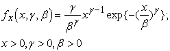 | (3.1) |
where γ is the shape parameter and β the scale parameter. When ϒ =1, the Weibull distribution is reduced to the exponential distribution with parameter λ = β.
The likelihood function for the Weibull distribution is given by:
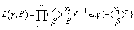 | (3.2) |
The log-likelihood function is therefore given by
 | (3.3) |
Thus, to determine the parameter estimates, we equate the derivatives of the log-likelihood function to zero and solve the following equations
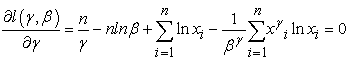 | (3.4) |
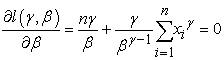 | (3.5) |
By eliminating β and simplifying, we obtained the following non-linear equation
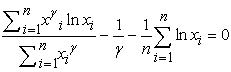 | (3.6) |
This can be solved numerically to obtain the estimate of ϒ by using the Newton-Raphson method. The MLE estimate for β is given by 
The Gamma distribution is a two-parameter family of continuous probability distributions and has a right skewed distribution. It is very useful for risk analysis modeling, particularly, for claims size modeling. It is extensions of the exponential distribution. It is expressed in terms of the gamma function which is defined by;
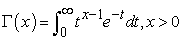 | (3.7) |
The probability distribution function (PDF) with two parameters is given by;
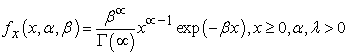 | (3.8) |
Where α>0 is the shape parameter and β>0 is the scale parameter.
The likelihood function for the gamma distribution function is given by
 | (3.9) |
The log-likelihood function is
 | (3.10) |
Thus, to determine the parameter estimates, we equate the derivatives of the log-likelihood function to zero and solve the following equations
 | (3.11) |
Thus
 | (3.12) |
Substituting  in the equation results in the following relationship for
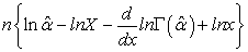 | (3.13) |
This result is a non-linear equation in  that cannot be solved in a closed form. This can be solved numerically using the root-finding methods.
The lognormal distribution is applicable to random variables that are constrained by zero but have a few very large values. The resulting distribution is asymmetrical and positively skewed. The application of a logarithmic transformation to the data can allow the data to be approximated by the symmetrical normal distribution, although the absence of negative values may limit the validity of this procedure.
Log normal distribution 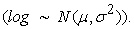 Parameter;
  The probability distribution is given by;
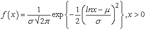 | (3.14) |
With parameters: location μ, scale σ > 0.
The likelihood function for the lognormal distribution is
 | (3.15) |
Therefore the log-likelihood function is given by
 | (3.16) |
The parameter estimator’s  and
and  for the parameters μ and σ can be determined by equating the derivatives of the log-likelihood function to zero and solve the following two equations
 | (3.17) |
And
 | (3.18) |
The resulting estimates are  and
and 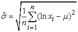 respectively.
With parameter α > 0 and γ > 0, is given by the distribution
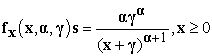 | (3.19) |
Where α > 0 represent the shape, and γ > 0 the scale parameter.
The likelihood function is
 | (3.20) |
The log-likelihood function
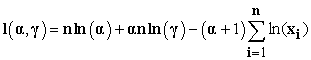 | (3.21) |
It is important to note that the best way to maximize the log-likelihood function is by adjusting as follows,  such that γ cannot be larger than the smallest value of x in the data. Thus, to determine the parameter estimate α equates the derivative of the log-likelihood function to zero we solve the following equations
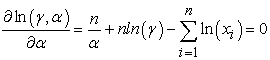 | (3.22) |
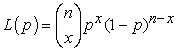
The binomial distribution is a popular discrete distribution for modeling count data. Given a portfolio of n independent insurance policies, let X denote a binomially distributed random variable that represents the number of policies in the portfolio that result in a claim. The claim count variable X can be said to follow a binomial distribution with parameters n and p, where n is a known positive integer representing the number of policies on the portfolio and p is the probability that there is at least one claim on an individual policy. The probability distribution function of X is defined as:
 | (3.23) |
The expected value of the binomial distribution is np and variance np(1- p). Hence, the variance of the binomial distribution is smaller than the mean. The corresponding binomial likelihood function is
 | (3.24) |
Therefore the log-likelihood function is
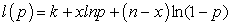 | (3.25) |
where k is a constant that does not involve the parameter p. Therefore, to determine the parameter estimate  we obtain the derivative of the log-likelihood function with respect to the parameter and equate to zero.
 | (3.26) |
Solving the above equation gives the MLE. Thus, the MLE is 
The Poisson distribution is a discrete distribution for modeling the count of randomly occurring events in a given time interval. Let X is the number of claim events in a given interval of time and λ is the parameter of the Poisson distribution representing the mean number of claim events per interval. The probability of recording x claim events in a given interval is given by
 | (3.27) |
A Poisson random variable can take on any positive integer value. Unlike the Binomial distribution which always has a finite upper limit. In general, the expected value and variance functions of the Poisson distribution are both equal λ. The Poisson likelihood function is
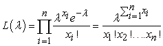 | (3.28) |
Therefore, the log-likelihood function is
 | (3.29) |
Differentiating the log-likelihood function with respect to λ, ignoring the constant term that does not depend on λ and equating to zero
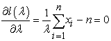 | (3.30) |
Solving the above Equation gives the MLE. Thus, the MLE is 
The negative binomial distribution is a generality of the geometric distribution. Consider a sequence of independent Bernoulli trials, with common probability p, until we get r successes. If X denotes the number of failures which occur before the rth success, then X has a negative binomial distribution given by
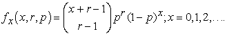 | (3.31) |
The negative binomial distribution has an advantage over the Poisson distribution in modeling because it has two positive parameters p > 0 and r > 0. The most important feature of this distribution is that the variance is bigger than the expected value. A further significant feature in comparing these three discrete distributions is that the binomial distribution has a fixed range but the negative binomial and Poisson distributions both have infinite ranges. The likelihood function is
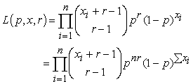 | (3.32) |
The log-likelihood function is obtained by taking logarithms
 | (3.33) |
Taking the derivative with respect to p and equating to zero.
 | (3.34) |
The resulting MLE estimate is  therefore, the negative binomial random variable can be expressed as a sum of r independent, identically distributed (geometric) random variables.
The Chi-Square goodness of fit test is used to test the hypothesis that the distribution of a set of observed data follows a particular distribution. The Chi-square statistic measures how well the expected frequency of the fitted distribution compares with the observed frequency of a histogram of the observed data. The Chi-square test statistic is:
 | (3.35) |
Where  the observed number of cases in interval j is,
  is the expected number of cases in interval j of the specified distribution and k is the number of intervals the sample data is divided into. The test statistic approximately follows a Chi-Squared distribution with k - p -1 degrees of freedom where p is the number of parameters estimated from the (sample) data used to generate the hypothesized distribution. A G-o-F test considers the null hypothesis that the sample data are taken from a population with the underlying distribution
  is rejected if the p-value is smaller than the criterion value at a given significance level α, at 5%.
The Anderson-Darling (A-D) test is an alternative to other statistical tests for testing whether a given sample of data is drawn from a specified probability distribution. This test gives more weight to the tails than Kolmogorov-Smirnov test which tends to be more sensitive near the center of the distribution than at the tails. Anderson-Darling (A-D) is given by the formula;
 | (3.36) |
Where  is the ordered sample of size n and
  is the underlying theoretical distribution to which the sample is compared. An A-D test is used to select the continuous claim severity distributions. Therefore, G-o-F tests consider null hypothesis that the sample data are taken from a population with the underlying distribution
  is rejected if the p-value is smaller than the criterion value at a given significant level α, at 5%.
The values of Akaike’s Information Criteria AIC were used to select the best model. Bayesian Information Criteria BIC can also be used to select best model but it has some limitation compared to AIC. Unlike AIC, BIC penalizes free additional parameters more strongly. AIC is good for making asymptotically equivalent to cross validation. On the contrary, BIC is good for consistent estimation. AIC tries to find unknown model that has high dimensional reality while BIC comes across only true models. For the above reasons AIC was the best for making inference from a sampled group of models. Therefore, the model with the smallest value of AIC was selected because this model is estimated to be closest to the unknown truth among models considered.
The AIC criterion is defined by:
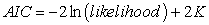 | (3.37) |
where K, is the parameter.
Frequency distribution was performed based on three models including binomial, Poisson and negative binomial distribution models. The results as shown in Table 1 below suggest that the p-values for the z-statistic in all the three models are less than 0.05 indicating that the parameter estimates for the three variables including the intercept are highly significant based on these models. Therefore, a significant relationship exists between the predictor variables and the response to frequency of the claims based on binomial, negative binomial and Poisson distributions models.
Moreover, the distributions of the residuals appear to be symmetrical in all the three models hence models predict all points closer to the actual observed points. The findings show that the null deviance for Poisson, Binomial and Negative Binomial distributions were found to be 1778.3, 1225.5 and 1202.08 respectively hence Negative Binomial distribution was considered to fit well as compared to Poisson distribution and Binomial distribution since it has a smallest value of the null deviance.
Parameter estimation was also done using Maximum Likelihood Estimation MLE method. The results show that LLF for Poisson, Negative Binomial and Binomial were found to be -1314.8528, -598.9715 and -1278.6367 respectively. From the results, it can be shown that the best model is Negative Binomial distribution with the highest value of LLF. This is further confirmed with AIC output where Negative Binomial distribution was found to be the best model since it has a smaller AIC value of 1205.9 as compared to both Poisson and Binomial distributions with 2637.7 and 2567.3 respectively. Hence, Negative Binomial distributions was considered as the best model for forecasting frequency of insurance claims. The results are summarized in Table 1 below.
4.2. Severity Claims ModelsSeverity of the claims was performed based on four models including Gamma, Weibull, Log normal and Pareto distributions. The results as shown in Table 2 below indicates that the p-values for the z-statistic in all the four models are less than 0.05 indicating that the parameter estimates for the five variables including the intercept are highly significant based on these models. Therefore, a significant relationship exists between the predictor variables and the response to severity of the claims based on Gamma, Weibull, log normal and Pareto distributions models.
The distributions of the residuals appear to be strongly symmetrical hence all models predict all points close to the actual observed points. The output of the fitted Null deviance for gamma distribution is 864.19 and residual deviance is 273.52. However, since Weibull, Pareto and Log normal distributions have no null deviance and residual deviance, Gamma distribution may be considered as appropriate model. However, the results of LLF based on MLE for Gamma, Weibull, Lognormal and Pareto distributions were found to be -10842.7846, -10986.1643, -10690.17 and -10346 respectively. From the results of parameter estimation, Pareto distribution was considered as the best model since it has highest value of LLF. This is further confirmed from the output of Akaike’s Information Criterion (AIC), where Gamma, Weibull, Log normal and Pareto distributions were found to have AIC values of 21703, 21988.96, 21396.33 and 20720.01 respectively thus suggesting that Pareto distribution with lower AIC value was considered the best model and for this reason, Pareto model was used in forecasting insurance severity claims. The results are presented in Table 2 below.
Chi-square goodness-of-fit test was performed in order to select the most appropriate claims frequency distribution among the fitted discrete probability distributions. The results as shown in Table 3 below suggest that the p-values for all the distributions including Poisson, Binomial and Negative Binomial distributions were less than 0.05 hence statistically significant. This confirms the above findings that Poisson, negative binomial and Binomial distributions were appropriate distributions for modeling frequency claims.
Anderson- Darling was performed in order to test the distributions used in modeling severity claims. The results as shown in Table 4 below suggest that p-values for Anderson-Darling test based on Gamma, Weibull, Log normal and Pareto distributions were less than 0.05 hence statistically significant. This indicates that strong evidence exists to support the hypothesis that Gamma, Weibull, Log normal and Pareto distributions were appropriate in modeling severity claims. However, Anderson-Darling test based on the CDF distance show that Pareto distribution was more appropriate than Gamma, Weibull and Log normal distributions hence concurs with the preference based on AIC values for all the datasets as Pareto distribution was also considered as the most appropriate claims severity distribution.
This section presents the results for the post model selection fit to affirm the selected models. 17, argued that the central problem in analysis is the kind of model one needs to use for making inferences from the claim dataset which is known as the model selection problem. As already shown and proven in both the selection criterion and the goodness of fit test above, the Pareto model emerged as the best fit for severity claims since it has least AIC and largest LLF. On the other hand, Negative Binomial distribution model emerged as the best fit for frequency claims since it has least AIC and largest LLF. It was also necessary to use goodness of fit criterion in order to select the severity model and frequency model that best fit the claim data. To obtain the expected amount of claims per risk for the following year, it was given by;  where
where  is the mean of the model selected.
The parameter estimates that were used to find expected frequency claim amount per risk is below.
Therefore, since Negative Binomial distribution was the best model for modeling frequency claims, mean of the model is 0.071. Hence, the expected amount of frequency claim per risk for the following year was 1.07372 1.
1.
Parameter estimates for severity distribution models that were used to find expected severity amount per risk is below.
Since Pareto distribution was the best severity model, with its parameters  and
and  mean of Pareto model is 8.7183. Hence, the expected claims amount per risk for the following year was Ksh 6,113.70.
The Pareto model was found to be the best fit model for the severity claim data among the four models tested. Anderson Darling test, AIC and LLF were used to measure the fitness of the model. The three tools confirmed, affirmed and reaffirmed that the Pareto model is the best fit model among the four models fitted. The expected claim amount per risk to be paid in the following year was estimated to be Ksh 6,310.70. On the other hand, Negative Binomial distribution model was found to best fit model for frequency claims data among models tested. The Chi-square test, AIC and LLF were used to measure the fitness, the three tools confirmed, affirmed and reaffirmed that Negative Binomial model is the best fit model among the three models fitted. The expected frequency claim amount per risk for the following year was estimated to be 1.07372 1. After a systematic study and going through actuarial modeling process by using comprehensive claim amount paid to policy holder and the frequency claims, the research concluded that Pareto model was the appropriate model for modeling comprehensive insurance claim severity with a heavier tail and Negative Binomial distribution model was the best appropriate model for modeling frequency claims of insurance company.
Since motor insurance is the fastest growing industry with overwhelming number of claims which are huge and unexpected, it is recommended that insurance companies use Negative Binomial model and Pareto model in forecasting of claims. This is because it assists insurance companies in their premium loading hence avoiding financial insolvency which threatens to place insurance companies under receivership. For further research, all models should be considered, which is critical. It’s also recommended that companies should use their own claims experience to make necessary adjustments to the models. This will allow for anticipated changes in the portfolios and for companies’ specific financial objectives. These proposed claims distributions will also be useful to insurance regulators in their own assessment of required reserve levels for various companies and in checking for solvency. It’s also recommended that further analysis should be done using models such as the zero-inflated models. This is because of large number of zeros in claims frequency data, hence there is need to consider other distributions such as the zero-truncated Poisson or zero-truncated negative binomial and zero-modified distributions to model this unique phenomenon.
| [1] | Lemaire, J. (2012). Bonus-malus systems in automobile insurance, volume 19. Springer science & business media. | ||
| In article | |||
| [2] | Tan, C. I., Li, J., Li, J. S.-H., and Balasooriya, U. (2015). Optimal relativities and transition rules of a bonus-malus system. Insurance: Mathematics and Economics, 61: 255-263. | ||
| In article | View Article | ||
| [3] | Klugman, S. A., Panjer, H. H., and Willmot, G. E. (2012). Loss models: from data to decisions, volume 715. John Wiley & Sons. | ||
| In article | View Article | ||
| [4] | Frees, E. W., Lee, G., and Yang, L. (2016). Multivariate frequency-severity regression models in insurance. Risks, 4(1):4. | ||
| In article | View Article | ||
| [5] | Garrido, J., Genest, C., and Schulz, J. (2016). Generalized linear models for dependent frequency and severity of insurance claims. Insurance: Mathematics and Economics, 70:205-215. | ||
| In article | View Article | ||
| [6] | Czado, C., Kastenmeier, R., Brechmann, E. C., and Min, A. (2012). A mixed copula model for insurance claims and claim sizes. Scandinavian Actuarial Journal, 2012(4): 278-305. | ||
| In article | View Article | ||
| [7] | Frees, E. W., Derrig, R. A., and Meyers, G. (2014). Predictive modeling applications in actuarial science, volume 1. Cambridge University Press. | ||
| In article | |||
| [8] | Shi, P., Feng, X., and Ivantsova, A. (2015). Dependent frequency-severity modeling of insurance claims. Insurance: Mathematics and Economics, 64:417-428. | ||
| In article | View Article | ||
| [9] | Park, S. C., Kim, J. H., and Ahn, J. Y. (2018). Does hunger for bonuses drive the dependence between claim frequency and severity? Insurance: Mathematics and economics, 83:32-46. | ||
| In article | View Article | ||
| [10] | Baumgartner, C., Gruber, L. F., and Czado, C. (2015). Bayesian total loss estimation using shared random effects. Insurance: Mathematics and Economics, 62: 194-201. | ||
| In article | View Article | ||
| [11] | Cheung, E., Ni, W., Oh, R., and Woo, J. (2019). A note on bayesian credibility with a dependent structure on the frequency and the severity of claims. Technical report, Working Paper. | ||
| In article | |||
| [12] | Lu, Y. (2019). Flexible (panel) regression models for bivariate count-continuous data with an insurance application. Journal of the Royal Statistical Society: Series A (Statistics in Society), 182(4):1503-1521. | ||
| In article | View Article | ||
| [13] | Anyanumeh, H. T. (2016). A suitable claim severity model of Comprehensive insurance policy. PhD thesis. | ||
| In article | |||
| [14] | Nelder, J. A. (1977). Are formulation of linear models. Journal of the Royal Statistical Society: Series A (General), 140(1): 48-63. | ||
| In article | View Article | ||
| [15] | Gourieroux, C., Monfort, A., and Trognon, A. (1984). Pseudo maximum likelihood methods: Theory. Econometrica: Journal of the Econometric Society, pages 681-700. | ||
| In article | View Article | ||
| [16] | Smyth, G. K. and Jørgensen, B. (1994). Fitting tweedie's compound poisson model to insurance claims data. In Scandinavian Actuarial Journal. Citeseer. | ||
| In article | View Article | ||
| [17] | Achieng, O. M. and No, I. (2010). Actuarial modeling for insurance claim severity in motor comprehensive policy using industrial statistical distributions. In International Congress of Actuaries, Cape Town, volume 712. | ||
| In article | |||
Published with license by Science and Education Publishing, Copyright © 2020 James Kiprotich Ng’elechei, Joel Cheruiyot Chelule, Herbert Imboga Orango and Ayubu Okango Anapapa
![]() This work is licensed under a Creative Commons Attribution 4.0 International License. To view a copy of this license, visit
http://creativecommons.org/licenses/by/4.0/
This work is licensed under a Creative Commons Attribution 4.0 International License. To view a copy of this license, visit
http://creativecommons.org/licenses/by/4.0/
| [1] | Lemaire, J. (2012). Bonus-malus systems in automobile insurance, volume 19. Springer science & business media. | ||
| In article | |||
| [2] | Tan, C. I., Li, J., Li, J. S.-H., and Balasooriya, U. (2015). Optimal relativities and transition rules of a bonus-malus system. Insurance: Mathematics and Economics, 61: 255-263. | ||
| In article | View Article | ||
| [3] | Klugman, S. A., Panjer, H. H., and Willmot, G. E. (2012). Loss models: from data to decisions, volume 715. John Wiley & Sons. | ||
| In article | View Article | ||
| [4] | Frees, E. W., Lee, G., and Yang, L. (2016). Multivariate frequency-severity regression models in insurance. Risks, 4(1):4. | ||
| In article | View Article | ||
| [5] | Garrido, J., Genest, C., and Schulz, J. (2016). Generalized linear models for dependent frequency and severity of insurance claims. Insurance: Mathematics and Economics, 70:205-215. | ||
| In article | View Article | ||
| [6] | Czado, C., Kastenmeier, R., Brechmann, E. C., and Min, A. (2012). A mixed copula model for insurance claims and claim sizes. Scandinavian Actuarial Journal, 2012(4): 278-305. | ||
| In article | View Article | ||
| [7] | Frees, E. W., Derrig, R. A., and Meyers, G. (2014). Predictive modeling applications in actuarial science, volume 1. Cambridge University Press. | ||
| In article | |||
| [8] | Shi, P., Feng, X., and Ivantsova, A. (2015). Dependent frequency-severity modeling of insurance claims. Insurance: Mathematics and Economics, 64:417-428. | ||
| In article | View Article | ||
| [9] | Park, S. C., Kim, J. H., and Ahn, J. Y. (2018). Does hunger for bonuses drive the dependence between claim frequency and severity? Insurance: Mathematics and economics, 83:32-46. | ||
| In article | View Article | ||
| [10] | Baumgartner, C., Gruber, L. F., and Czado, C. (2015). Bayesian total loss estimation using shared random effects. Insurance: Mathematics and Economics, 62: 194-201. | ||
| In article | View Article | ||
| [11] | Cheung, E., Ni, W., Oh, R., and Woo, J. (2019). A note on bayesian credibility with a dependent structure on the frequency and the severity of claims. Technical report, Working Paper. | ||
| In article | |||
| [12] | Lu, Y. (2019). Flexible (panel) regression models for bivariate count-continuous data with an insurance application. Journal of the Royal Statistical Society: Series A (Statistics in Society), 182(4):1503-1521. | ||
| In article | View Article | ||
| [13] | Anyanumeh, H. T. (2016). A suitable claim severity model of Comprehensive insurance policy. PhD thesis. | ||
| In article | |||
| [14] | Nelder, J. A. (1977). Are formulation of linear models. Journal of the Royal Statistical Society: Series A (General), 140(1): 48-63. | ||
| In article | View Article | ||
| [15] | Gourieroux, C., Monfort, A., and Trognon, A. (1984). Pseudo maximum likelihood methods: Theory. Econometrica: Journal of the Econometric Society, pages 681-700. | ||
| In article | View Article | ||
| [16] | Smyth, G. K. and Jørgensen, B. (1994). Fitting tweedie's compound poisson model to insurance claims data. In Scandinavian Actuarial Journal. Citeseer. | ||
| In article | View Article | ||
| [17] | Achieng, O. M. and No, I. (2010). Actuarial modeling for insurance claim severity in motor comprehensive policy using industrial statistical distributions. In International Congress of Actuaries, Cape Town, volume 712. | ||
| In article | |||


