1. Introduction

So many studies have been done about systematic sampling (Kish ^[1], Cochran ^[3], Särndal et al. ^[4], Sharon ^[5], Thompson ^[6], Groves et al. ^[7]). In this paper, on a basis of former studies, I propose a new model of systematic sampling, which procedure is a little bit different from the former ones, and try giving a theory. The model, which I call Roulette Model, can be executed easily and enables us to calculate the expectation of statistic exactly as it is.

Let us consider a problem to select n out of N elements by systematic sampling.

When is an integral multiple of the sampling interval is also an integer. If a random start is drawn from 0 to the sample is determined by

(1.1.1)

elements in a population list for But is given at first and what we can decide is only What if is a prime number? In general, is not necessarily an integer and problems with the sampling intervals will arise.

By Kish ^[1], the following four solutions were given (pp. 115-117).

1. Permit the sample size to be either or .

2. Eliminate with epsem (equal probability of selection method).

3. Consider the list to be circular.

4. Using fractional intervals.

He wrote “the sampler should choose the most convenient”. Cochran ^[3] gave an integral sampling interval at first and permitted the sample size to change (pp. 205-206). He also introduced a method suggested by Lahiri ^[8] (see Murthy^[2] p. 139). Särndal et al. ^[4] organized the former studies and gave the definitions and main results. Anyway, the sampling procedures are optional.

On a basis of former studies, I will arrange and reconstruct the procedure of systematic sampling in my own way as follows. Let us draw a numerical line across N●-points.

Let the random start be a random number over and consider the population list to be circular.

And decide the sample by

(1.2.1)

elements in the list for The problem lies in the case when is not an integer. Which should I select

(1.2.2)

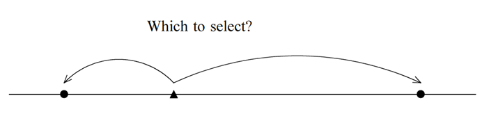In a sampling problem, I don't think it essential whether is an integer or not. I also think it unnatural that only the first sampling point (when ) is always an integer. Since is not necessarily an integer, the procedure of systematic sampling should be considered as a continuous problem. The following concept seems to be the most natural for me.

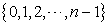
i. Draw two circles with the same length of circumference N. On one, put N●-points

with the same interval 1 and set the point 0 at the top. On another, put n▲-points

with the same interval and setthe point 0 at the top. It doesn't matter whether is an integer or not.

ii. Rotate the latter circle by random angle along the circumference like roulette.

iii. And lap it over the former one.

iv. As a sample, choose ●-points correspondent to where ▲-points dropped.

This simple procedure above is a concept of Roulette Model. It can be formulated as follows.

2. Formulation

In this paper, I assume all functions are defined on . That is, if a parameter of a function is outside of the interval

(2.1.1)

I add or subtract by necessary times so as to settle it within .

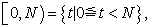
i. A circle with the length of circumference can be regarded as an interval . So I identify the population list with an interval .

ii. As the interval is a disjoint union of unit intervals

(2.2.1)

I identify an element in a population list with a unit interval

(2.2.2)

iii. If a ▲-point belongs to , select as an element of sample. Here I don't require any relation between and . So, when can be selected repeatedly the same times as the number of ▲-points which belong to .

In the above procedure, I used a random angle, which is a uniform random number over an interval

(2.3.1)

Along the circumference, this is equivalent to a uniform random number over an interval

(2.3.2)

I consider producing the latter from now on.

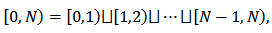
As an interval is a disjoint union of unit intervals

(2.3.3)

I consider producing two independent random numbers and as

(2.3.4)

Here is a discrete uniform random number over and is a continuous uniform random number over Then will surely be a uniform random number over

(2.3.5)

By , I select a unit interval among intervals And by , I focus on a point in the selected interval. That is, I decide a random number over in two steps.

In Roulette Model, I decide the first sampling point not by but by identify an element in a population list with a unit interval and choose when

(2.4.1)

for Then

(2.4.2)

elements for re selected as a sample because

(2.4.3)

The existence of -term is a different point from the former procedures. By contribution of -term, even if the same first sample and the same sampling interval are given, stilla different sample can be selected when neither nor is an integer.

3. Calculation

The greatest advantage of Roulette Model is, just by adding -term, to enable us to calculate the expectation of statistic exactly as it is.

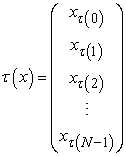
Assume that our interest is value The population is described as

(3.1.1)

and the sample is described as

(3.1.2)

Given and , the sample is decided. Considering any statistic written by

(3.1.3)

as is known from how we produced two random numbers its expectation is calculated by

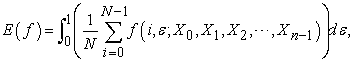(3.1.4)

where the order of summation and integral is commutative.

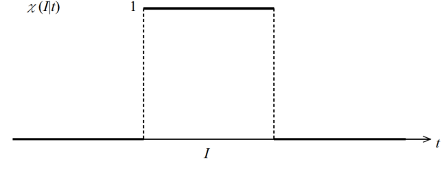
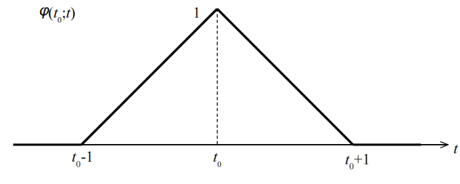
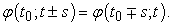
I define a characteristic function and a pulse function by

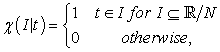(3.2.1)

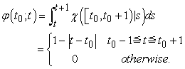(3.2.2)

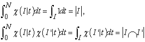
For an interval 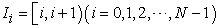, I write

(3.2.3)

Then it leads

(3.2.4)

Considering the meaning of and , we obviously have the following lemmas.

Lemma 1. For any integer ,

(3.2.5)

Lemma 2.

(3.2.6)

Lemma 3.

(3.2.7)

Lemma 4. For any real number ,

(3.2.8)

Lemma 5.

(3.2.9)

Let the population mean and the population variance

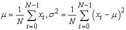(3.3.1)

respectively.

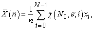
Given and the sample is decided. So we can regard the sample as a function of and, by the meaning of we have

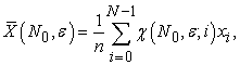
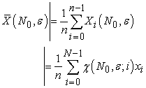(3.3.2)

as a sample mean. By lemma 1 and 2, we can calculate its expectation as follows.

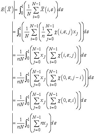(3.3.3)

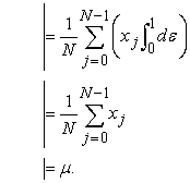(3.3.3)

We hereby get the proof of unbiasedness of sample mean by systematic sampling. As is known from the above process of calculation, -term does not contribute at all. So unbiasedness still holds when

Theorem 1. Sample mean by systematic sampling is an unbiased estimator of population mean.

(3.3.4)

In an identity

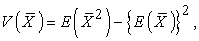(3.4.1)

we have the relation

(3.4.2)

so we have

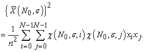(3.4.3)

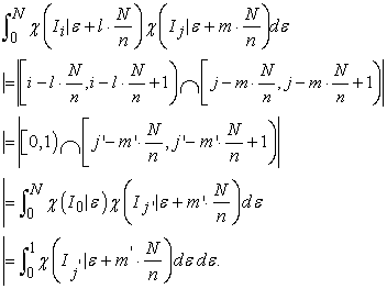
The expectation is calculated by

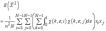(3.4.4)

By the definition of , we get

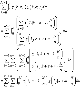(3.4.5)

Here, if we put

(3.4.6)

by lemma 3, we have

(3.4.7)

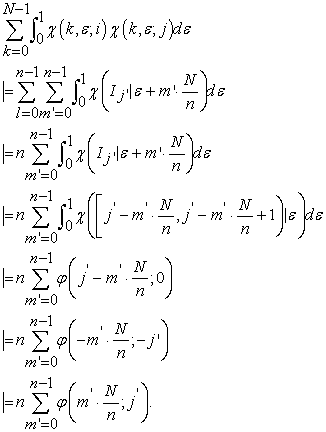(3.4.8)

At last, we obtain

(3.4.9)

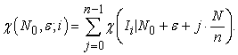
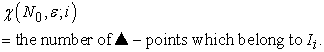
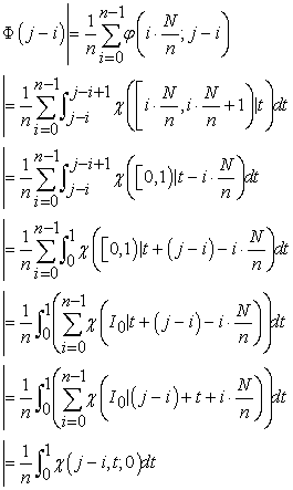
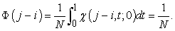
Here I define a function by

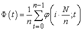(3.4.10)

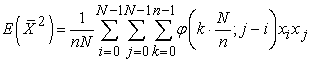
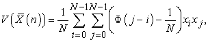
and get the explicit description of the variance of sample mean as

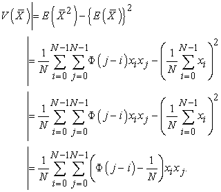(3.4.11)

Theorem 2. The variance of sample mean by systematic sampling is described as

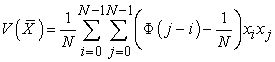(3.4.12)

That a function has a parameter means that depends on how to sort a population list.

The expectation of sample variance

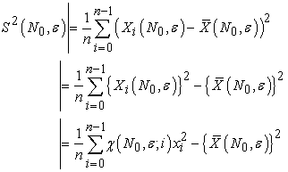(3.5.1)

is calculated, by lemma 1, 2 and 3, as

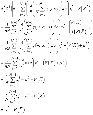(3.5.2)

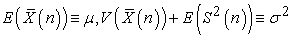
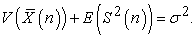
In general, sample mean and sample variance can be regarded as functions of sample size . So I write them and respectively from now on. From the result of 3-5, in systematic sampling,

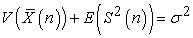(3.6.1)

holds. On the other hand, in random sampling with replacement,

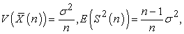(3.6.2)

so we have

(3.6.3)

In random sampling without replacement, because

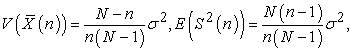(3.6.4)

we again have

(3.6.5)

While and are random variables, and are constants. In general, 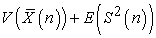is considered to depend on sample size n and how to select a sample. So the above results tell us the conserved quantity between random and systematic sampling.

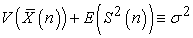
Theorem 3. Between random and systematic sampling, the following quantities are conserved.

(3.6.6)

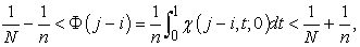
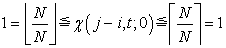
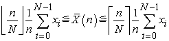
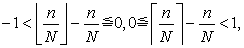
In

(3.7.1)

from lemma 5, we immediately have inequalities

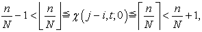(3.7.2)

(3.7.3)

so we obtain

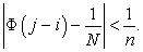(3.7.4)

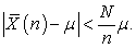
Applying this estimation to

(3.7.5)

we get an analogy of law of large numbers.

Theorem 4. In systematic sampling, while

(3.7.6)

is kept,

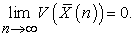(3.7.7)

Moreover, while we obviously have

(3.7.8)

for random sampling without replacement, we also have

(3.7.9)

for systematic sampling because, when

(3.7.10)

and

(3.7.11)

That is, of systematic sampling has both properties of random samplings with and without replacement.

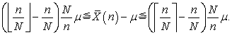
When is nonnegative and , from (3.7.4), we can estimate

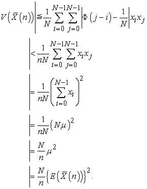(3.7.12)

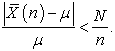
So the coefficient of variation of is less than

Corollary 1. When is nonnegative and

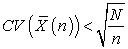(3.7.13)

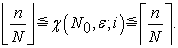
Applying lemma 5 to

(3.7.14)

we get the following estimation.

(3.7.15)

and

(3.7.16)

Here, as

(3.7.17)

we have

(3.7.18)

This result suggests the robustness of systematic sampling.

Corollary 2. When is nonnegative and

(3.7.19)

4. Discussion

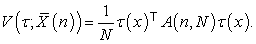
Define a vector and an matrix as

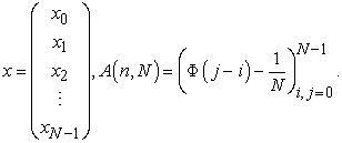(4.1)

Then can be regarded as a quadratic form

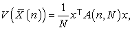(4.2)

where s obviously a positive semi definite matrix.

Proposition. For any and any real vector

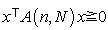(4.3)

and

(4.4)

How to sort a population list is nothing but how to permutate a population list mathematically. So, if I write

(4.5)

for where is a permutation group of degree can be regarded as a function of and written as

(4.6)

Here the next question will arise.

What kind of givesless ?

Obviously the value is conserved according to a cyclic permutation. I leave this problem to the readers. Thank you so much for reading my poor English to the end.

Acknowledgement

I would like to express my gratitude to Reiji Murayama and Yoshihiro Yumiba for their sincere encouragement. Also I would like to extend my indebtedness to Takashi for his endless love, understanding, support and encouragement throughout my study. The responsibility for any errors is entirely mine.

References

[1]	Leslie Kish, Survey Sampling, John Wiley & Sons, Inc., 1965.
	In article
[2]	Murthy, M. N., Sampling Theory and Methods. Statistical Publishing Society, Calcutta, India, 1967.
	In article
[3]	William G. Cochran, Sampling Techniques, John Wiley & Sons, Inc., 1977.
	In article
[4]	Carl-Erik Särndal, Bengt Swensson and Jan Wretman, Model Assisted Survey Sampling, Springer, 1992.
	In article		CrossRef
[5]	Sharon L. Lohr., Sampling: Design and Analysis. Duxbury Press, 1999.
	In article
[6]	Steven K. Thompson, Sampling, John Wiley & Sons, Inc., 2002.
	In article
[7]	Robert M. Groves, Floyd J. Fowler, Jr., Mick P. Couper, James M. Lepkowski, Eleanor Singer, and Roger Tourangeau., Survey Methodology. John Wiley & Sons, Inc., 2004.
	In article
[8]	Lahiri, D. B., “A method for sample selection providing unbiased ratio estimates”. Bull. Int. Stat. Inst., 33, 2, 133-140, 1951.
	In article