Every year there were regular atmospheric oscillation representing in the form of convection and precipitation. This article elicits the fluctuations in atmospheric oscillation which have been modulated by various atmospheric effects altering convection in different regions over India. The semi-annual and annual oscillation occurring in the atmosphere can be observed through some atmospheric indices. To assess the amplitude and frequency of these oscillations, we have used atmospheric index i.e Lifted index over six regions, New Delhi, Mumbai, Kolkata, Hyderabad, Bengaluru and Chennai for the duration January 1996 to December 2016. To extract information we have implemented Singular Spectrum Analysis which decomposes data and to find amplitude and frequency we implemented Fast Fourier Transformation. From FFT it is observed that the annual and semiannual amplitudes of Lifted Index of six stations lie between 2°C to 6°C and 1.5°C to 2°C respectively. Kolkata has annual amplitude value of 6.041°C and semiannual amplitude value of 3.643°C which are more as compared to other stations. Chennai has least annual amplitude value of 2.403°C and Bengaluru has least semiannual amplitude value of 1.342°C. Even though Kolkata and Chennai are coastal regions near Bay of Bengal, variation in maximum and minimum magnitudes of Kolkata are more as compared to Chennai and hence Kolkata might have more convection and precipitation. The results from this study are mostly consistent with the previous studies. A detailed inferences of these results are discussed.
The basis of the atmospheric climate discrepancies over different regions in the Earth’s atmosphere is due to solar heating of the planet, atmosphere, ocean, land and ice responses to heating, difference in pressure and temperature consequently persuade in the form of precipitation 1, 2. India, being different in geographic conditions has diverse climate with various amplitude in atmospheric oscillations and precipitations over the regions. Indian climate is a dynamical system which is also biased by many external factors for instance solar radiation, geographical conditions surrounding the regions with apparently significant phenomena like cyclones overlapping on the regions. Infact, Indian region is covered with the Himalayas in northern part and the other three sides are covered by oceans thereby influencing a range of pressure and temperatures over the region. The progress of these atmospheric phenomena are guided by many physical principles which can be put carefully in an efficient and useful way for wellbeing of nature. These effects of climatic changes having significant phenomena on annual and semiannual seasons compel to study for persisting living things.
The research on climate variations always played a crucial role along with the other scientific disciplines imparting important relationship among atmospheric parameters with objectives in their study. The enigma of the Indian monsoon and its notable regularity over a given time interval depart from one region to the other with distinguished periodicities 3, 4, 5. These periodicities is the essence of our study. Few researchers have revealed atmospheric oscillations with different techniques and with different data. Ramamurthy studied Indian summer monsoon with characteristics of active and break spells of monsoon rainfall and revealed ISM as intraseasonal oscillations within the summer monsoon season 6. These active and break spells of the monsoon are associated with fluctuations of the tropical convergence zone expressed by Sikka and Gadgil and also by Yasunari, 7, 8. Mehta and Krishnamurti also examined the interannual variability of the 30-50 day mode using characteristics of northward propagation of the winds at 850 and 200 hPa for the period 1980-84 9. Singh and Kripalani observed 30-50 day oscillation in Indian monsoon variation using long duration daily rainfall data 10. Goswami and Mohan, studied Intraseasonal Oscillations and Interannual Variability of the Indian Summer Monsoon and observed annual and semiannual oscillations in zonal winds at 850 hPa 3. By knowing all the factors related to atmosphere like solar influx, Relative humidity, Pressure, Temperature, level of free convection, equilibrium level, Lifted, Showalter, K, Total Totals Index, Convective Available Potential Energy, Convective Inhibition etc., affecting the atmospheric conditions at a given time with complete statistical uncertainty details through non linearities and instabilities it will be better to predict the state of the climate system over the given regions.
The unpredictable atmospheric conditions having different features at different times over different regions are furnished through certain noteworthy atmospheric instability indices like Lifted index (LI) 11, Showalter index (SI) 12, K index (KI) 13, Total Totals index (TTI), convective inhibition, CAPE etc 14, 15 and few of these indices studied by researchers. These indices which evolve with all effects within them allows us to interpret the linear, regular and non linear variations through certain techniques with determined set of amplitudes.
The atmospheric stability indices bring forth very essential features in forecasting and is useful to observe the events of instability in the atmosphere at a specific time. In this study we have determined frequent occurrences of oscillations and the set of amplitudes of annual and semiannual oscillations variations using atmospheric lifted index data at six different climatic regions over India. LI describes convective activity in the atmosphere and a useful forecast means for predicting latent instability. Galway on examination of the atmospheric soundings data reveals LI is a useful forecast tool for the prediction of latent instability 11. Positive values of this index reveals stable atmosphere without any convection. Negative values correspond to unstable atmosphere guiding towards higher convective activity. The range of negative values of LI between −4°C and −8°C indicates more convection thereby having chances of thunderstorm occurrences. Early investigations explained in relation to these four indices were somewhat more or less represented. The majority of researcher paid attention on the analysis of atmospheric indices either annually or seasonally or for a particular region. As mentioned above that India’s geographical position is diverse in the world and require a detail study at one site to get correct picture of variation of atmospheric indices as a whole.
This paper presents data availability, data description, its quality checks, materials and methods in section 2 and results pertaining to this study in section 3.
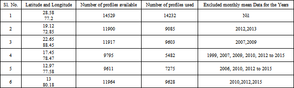
The data collected in the present study for the above mentioned index from Integrated Global Radiosonde Archive (IGRA) available at (https://www.ncei.noaa.gov/pub/data/igra/data) for the duration January 1996 to December 2016. The data description and analysis on data have been performed quality checks and used by many researchers 16, 17, 18, 19. In this study we have selected six stations New Delhi, Mumbai, Kolkata, Hyderabad, Bangalore and Chennai over India. The available profiles and excluded dataset were mention in the below Table 1. There were data gaps which are within the month for New Delhi, the data gaps were not found to be significant for monthly mean data set with respect to span of (21 years X 12 months) the data 19 and for the remaining station we have studied annual and seasonal oscillations only for the available monthly mean data and for the continuous duration. For the daily IGRA data, we have calculated daily mean and mean for every month for all year and for all the stations. To observe seasonal oscillations in daily mean data we have implemented Singular Spectrum Analysis (SSA) method and applied Fast Fourier transformation (FFT) technique to observe frequency and amplitude in the oscillations.
Singular Spectrum Analysis (SSA) is a non-parametric, comparatively quite recent and indepth technique for time series analysis and prepared with the purpose of extracting oscillations, detrending in time series and to remove obstructions in suitable many existing problem which is functional to several sensible like signal and noise processing 20, 21. This method is widely used in many applications such as signal processing which provides qualitative and quantitative information about the deterministic parts of the system in time series with noise, Vautard and Ghil 22. The behaviour and features of SSA like window length, sampling interval and length of samples have been implemented. Vautard and Ghil also describe that the results of SSA which extract vital components and spectral characteristics are useful for the interpretation of data set. Sharma et al., calculated low dimensionality using SSA while studying global magnetospheric dynamics 23. The relation between Indian monsoon, the North Atlantic ocean (NAO) and the Southern Oscillation Index for Tropical Pacific investigated with spectral peaks using SSA by Yizhak Feliks, Andreas Groth, Andrew W. Robertson and Michael Ghil 24. Using SSA method the time series can be decomposed into trends, different oscillations and noise by Ghil et al., 25. The singular spectrum analysis (SSA) is useful to analyse time series data of many disciplines in which the data is decomposed into orthogonal components which exhibits trends and oscillatory patterns 20, 21, 25, 26. In general oscillations having frequency, phase and amplitude modulated are superimposed with each other and using this SSA method we are extracting annual and semiannual oscillations from seasonal time series signal. The outcome of this work is practicable and harmonizing in pulling out required information from the time series and constructive way to interpret oscillations in lifted index for six different regions and to demonstrate SSA method. These extracted different oscillations should be distinguished in order to recognize the essential features in environmental and atmospheric processes. To a large extent we have focussed in understanding seasonal signals that are coupled with several resources.
The algorithm of SSA includes the different stages, they are (a) Construction of covariance or trajectory matrix (b) calculating SVD (c) Grouping of SVD (d) Reconstruction of covariance matrix. There were few processes in SSA method. The first process is arranging the given time series into covariance matrix or Hankelisation. Let us take a time series TN = (f0, . . . , fN−1) of length N which is sum of several unknown, irregular but identifiable oscillations. While converting a time series into trajectory matrix we use window length L. By using window length L (1 < L < N) we construct K = N − L + 1 lagged vectors Xi = (fi−1, . . . , fi+L−2), where 1 ≤ i ≤ K, and constructed trajectory matrix X = [X1 : . . . : XK], which is also called Hankel or Covariance matrix whose diagonal elements remains same. The eigen values and eigen vectors of this Covariance matrix were calculated. Using these eigen values and eigen vectors we calculate principal components and finally computed reconstructed components from the decomposed time series as described by many researchers 20, 21, 22, 25, 26, 27, 28, 29.
Initially we observe seasonal component for daily mean LI raw data for New Delhi regions and for the above mentioned duration. Observed periodicities in LI for the six regions. Next we have applied SSA to decompose and to find reconstructed components and then applied FFT to the reconstructed components. The time series of LI of New Delhi for the duration January 1996 to December 2016 is examined by taking window length of 360 days for daily mean data, window length of 12 and 120 months for monthly mean data. Selection of window length depends on the data and the aim of accomplishment of analysis 20, 21, 30. In general the window length is taken half the total data length (L) and smoothing of the series can be performed with small values of L 30. In this study we have selected window length (L=12 and 120 for monthly mean and 360 for daily mean) to extract a periodic component with known period, which are very small as compared to the dataset but multiples of periodic components as we are looking only for annual and semiannual oscillations. The window length L=360 is taken for daily mean only to observe smoothness of the first RCC. The eigenvalue spectra for window length L=12 and 120 have been calculated for monthly mean data of New Delhi for the above mentioned duration. The eigenvalue spectra for two window length have been depicted for different modes to observe its contribution for trajectory matrix. When more eigenvalues are added the cumulative percentage of variance increases and for five eigenvalues we have observed 90% of contribution for the covariance matrix. Extracted trend component and noise from reconstructed matrix.
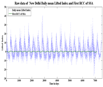
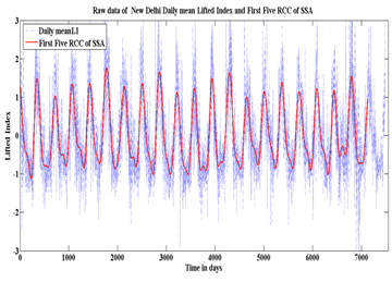
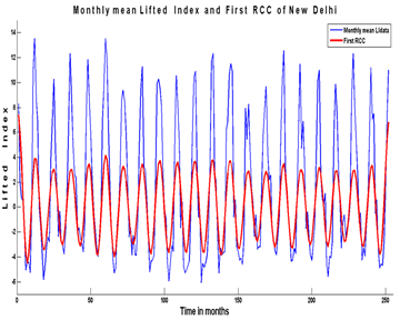
Daily mean and its first reconstructed components (RCC) of New Delhi LI for the duration January 1996 to December 2016 is depicted as shown in Figure 1. From Figure 1 it is noticeable that the first RCC calculated using SSA shows annual oscillation but with low amplitude. It is also observed that the calculated first five RCC of SSA is shown in Figure 2 and is apparent that the sum of first five RCC’s were put up in close to the daily mean data indicates that each RCC is the harmonic having different amplitude and frequency. The daily mean data is used to observe how far the SSA’s RCC smoothens the data. In this study we have retrieved these harmonics using SSA and investigated the possibility of their amplitudes. Using this method we have extracted and identified the core patterns in the data in the order of decreasing amplitudes.
In this SSA method the time series is embedded to make covariance matrix by using different window lengths L. The eigen values and eigen vectors, principal components and reconstructed components have been calculated for this covariance matrix. The eigenvalues calculated using covariance matrix are arranged in decreasing order. These eigenvalues represents the variance of the data set relating to eigenvector which explains more values of eigenvalue has more variance for that specific component 22. First two eigen values are nearly equal and periodic observed by Plaut and Vautard 31. Schoellhamer used SSA method to obtain spectral estimates 29. Furthermore Ghil, Allen, Dettinger, Kondrashov, Mann, Robertson, Saunders, Tian, Varadi, and Yiou anticipated in selecting window length in order to extract information in series 26. In this study we have taken three window lengths in spectral point of view. One for daily mean data, the window length is 360 data points to observe smoothness of RCC components which is depicted in Figure 1 and the other two for monthly mean data whose window length is 12 and 120 data points to observe annual and semiannual periodic components which is depicted in Figure 5 and Figure 9.
The core function of SSA is decomposition of the time series into several periodic components, trend and noise 20. It is based on the singular value decomposition of a trajectory matrix constructed with the data set. For the daily mean with L=360 we have observed first RCC, which contributes only feeble amount of covariance matrix, as the trend which can be noticed in Figure 1. We have also observed that the sum of five reconstructed components of series, which contributes about 60% of covariance matrix, which is in close resemblance to the oscillations of the data which is shown in Figure 2. The eigenvalue spectra for daily mean series is not depicted here.
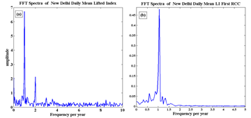
The daily mean LI raw data of New Delhi is applied to FFT and observed annual and semiannual periodicities as depicted in Figure 3 in which frequency per year on x-axis and amplitude on y-axis. It is observed that there are two significant peaks, one at frequency of 1 per year with amplitude 6.722°C which indicates annual period and second at frequency of 2 per year with amplitude 2.127°C which indicates semiannual period.
From reconstructed components for the daily mean data it is observed that there are different components having different frequencies. These different frequency components have been extracted and detected periodicities by applying FFT.
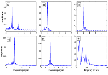
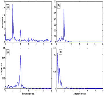
The FFT spectra of sum of first five RCC’s daily mean LI is depicted in Figure 4a. From Figure 4a it is clearly evident that there are two significant peaks, one at frequency 1per year and second at frequency 2per year and it can be noticed that the second component has low amplitude. From this we can conclude that semiannual oscillations could be in the first five RCC components. It is also noted that the first five individual RCC’s FFT spectra are shown in Figure 4b to Figure 4f. From this figure it is evident that the amplitudes are decreasing. From Figure 4b and Figure 4c the frequencies are 1 per year with decreasing amplitude. From Figure 4b and Figure 4c it can be concluded that there were two annual oscillations which are coupled having different amplitude. Similarly from Figure 4d and Figure 4e the frequencies are 2 per year with decreasing amplitude, indicating that there were lower amplitude semiannual oscillations present in the lifted index. Similarly from Figure 4d and Figure 4e it can be concluded that there were two semiannual oscillations which are coupled having different amplitude. From Figure 4f it is observed that there are three peaks with lower frequencies less than 0.5 per year. It can concluded that the oscillations having frequencies less than 0.5 per year might be due to local regional influence in the atmosphere.
Applied SSA with window length L=12 for monthly mean data in order to decompose and find periodic components. Figure 5 shows monthly mean data and its first RCC and Figure 6 shows monthly mean data and its sum of first four RCC’s.
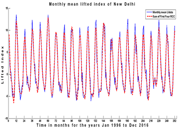
The covariance matrix generated from the data set using SSA by window length can be approximated using singular value decomposition and by making use of RCC’s, which has more contribution to the trajectory matrix, we can extract trend in the data set 20, 22. In this study we have applied SSA with L=12 for the monthly mean lifted index to all stations for the available data in the duration Jan 1996 to Dec 2016. Here we have depicted the sum of first four RCC’s having more contribution for the covariance matrix for New Delhi as shown in Figure 6.
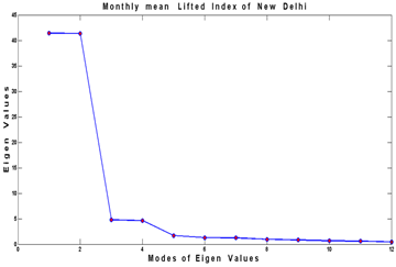
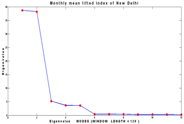
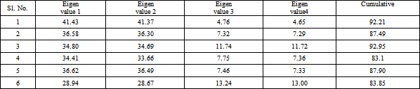
The eigen values of covariance matrix with L=12 for the monthly mean lifted index of all stations for the mentioned duration have been calculated. The first four eigenvalues has nearly 80 to 90% contribution to the covariance matrix. The first four eigenvalue’s relative and cumulative contribution in percentage were tabulated in Table 2. The eigen values of covariance matrix with L=12 for the monthly mean lifted index of New Delhi for the mentioned duration is depicted in Figure 7. From this Figure 7 it is observed that the first two eigen values are nearly equal and sum of first four eigen values contributes upto 92% of the total variation of the series. Here we have shown figure of eigen value spectra only for the New Delhi but the remaining stations also has the similar variation upto 12 eigen values which are tabulated only for four eigenvalues in Table 2. From Table 2 we have observed that the first two eigen values has more relative contribution as compared to third and fourth.
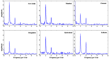
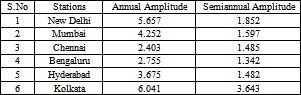
The FFT is applied to sum of four RCC’s and individual RCC’s decomposed from SSA of monthly mean of LI of New Delhi which is depicted in Figure 8. It is observed that the annual and semiannual periodicities have different amplitudes. Comparing the daily mean we have noticed similar patterns for monthly mean data which is shown in Figure 8a to Figure 8d. It is noticed even in monthly mean data there is no difference in amplitude and frequency. And also observed annual and semiannual periodicity in remaining stations with similar pattern but not shown in this study. The FFT applied to sum of four RCC’s of monthly mean of LI of six stations were also shown in Figure 9. It is observed that Kolkata has more amplitude value of 6.041°C in annual oscillation and semiannual amplitude value of 3.643°C as compared to other stations. The amplitude values from FFT spectra of monthly mean LI of six stations have been tabulated in Table 3. Among annual amplitudes Chennai has least annual amplitude value of 2.403°C and Bengaluru has semiannual amplitude value of 1.342°C which is a low value as compared to other stations. The FFT spectra of daily mean LI of New Delhi is shown in Figure 4 and monthly mean LI is shown in Figure 8. When compared to daily mean LI and monthly mean LI of New Delhi there is slight variation in amplitude due to variation in eigenvalues.
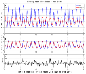
The SSA is also performed for the window length 120 which is near to half of total data length and depicted the RCC’s and eigenvalue spectra in Figure 10 and Figure 11 respectively for monthly mean lifted index of New Delhi. Figure 10a shows monthly mean lifted index in blue and the first RCC in red curve whose eigenvalue contributes nearly 40% to the covariance matrix indicating the trend of the data. Figure 10b shows sum of the first five RCC’s in red curve indicating more than 90% contribution of eigenvalues in reconstruction. Figure 10c shows the noise.
The percentage contribution of eigenvalues to the trajectory matrix with L=120 for monthly mean lifted index of New Delhi is depicted as shown in Figure 11. It is observed that even with L=120 only the first five RCC’s has more contribution with respect to the remaining. We have observed similar pattern of eigenvalue spectra for the remaining stations but not shown here.
The time series can be decomposed into different components having different frequencies using SSA method by selecting proper window length. The eigen values and eigen vectors have been calculated to reconstruct components. It is also observed that the two consecutive eigen vectors are orthogonal to each other. Observed trend showing annual periodicity in the first RCC. Observed only the first five eigenvalues has more contribution to the trajectory matrix in the eigenvalues spectra for two different window length. The sum of first five RCC’s of both daily and monthly mean nearly resembles the raw data have been depicted. From FFT spectra of daily, monthly mean, sum of first five RCC’s and individual RCC’s annual and semiannual periodicities have been observed. Observed significant differences in amplitudes of annual and semiannual oscillations in LI between regions related to the same coastal influence.
The author thanks the Principal, KVR Government College for Women (A), Kurnool, A.P. India, for providing technical support. The author is thankful to all the faculty members of School of sciences, Maulana Azad National Urdu University, Hyderabad, India, for their encouragement. She also acknowledges National Atmospheric Research Laboratory (NARL), India, for providing necessary support for this work and data obtained on request. Grateful thanks are also due to an anonymous reviewer for the valuable comments that helped to improve the paper.
| [1] | Loubere, P. (2012). The Global Climate System. Nature Education Knowledge”, 3(10): 24. | ||
| In article | |||
| [2] | Trenberth.KE, JT Houghton, and LG Meira Filho,( 1996), “Climate system: An overview: CLIMATE CHANGE 1995 THE SCIENCE OF CLIMATE CHANGE”., CAMBRIDGE UNIVERSITY PRESS, NEW YORK, NY (USA), pp. 51-64. | ||
| In article | |||
| [3] | Goswami, B. N., and R. S. Ajaya Mohan (2001), “Intraseasonal oscillations and interannual variability of the Indian summer monsoon”, Journal of Climate, 14. | ||
| In article | View Article | ||
| [4] | Government of India, Ministry of Earth Sciences, India Meteorological Department, “Salient Features of Monsoon 2021”, Press Release,1st October, 2021 | ||
| In article | |||
| [5] | Nityanand Singh and Ashwini A. Ranade, (2010), “Determination of Onset and Withdrawal Dates of Summer Monsoon across India using NCEP/NCAR Re-analysis”, 10.13140/RG.2.1.2059.5367. | ||
| In article | |||
| [6] | Ramamurthy, K (1969), “Monsoon of India: Some aspects of ‘break’ in the Indian south west monsoon during July and August”. Forecasting Manual, Report IV, Vol. 18. | ||
| In article | |||
| [7] | Sikka, D. R., and S. Gadgil (1980), “On the maximum cloud zone and the ITCZ over Indian longitudes during the southwest monsoon”, Mon. Wea. Rev., 108, 1840-1853. | ||
| In article | View Article | ||
| [8] | Yasunari, T. (1979), “Cloudiness fluctuation associated with the Northern Hemisphere summer monsoon”. J. Meteor. Soc. Japan, 57, 227-242. | ||
| In article | View Article | ||
| [9] | Mehta, V. M., and T. N. Krishnamurti (1988), “Interannual variability of 30-50 day wave motion”. J. Meteor. Soc. Japan, 66, 535-548. | ||
| In article | View Article | ||
| [10] | Singh, S. V., and R. H. Kripalani (1990), “Low frequency intraseasonal oscillations in Indian rainfall and outgoing long wave radiation”. Mausam, 41, 217-222. | ||
| In article | |||
| [11] | Galway, J.G., (1956), “The lifted index as a predictor of latent instability.” Bull. Amer. Meteor. Soc., 37, 528-529. | ||
| In article | View Article | ||
| [12] | Showalter.A. K. (1953), “A Stability Index for Thunderstorm Forecasting”, Bulletin of the American Meteorological Society, Vol. 34, No. 6, pp. 250-252. | ||
| In article | View Article | ||
| [13] | George, J. J., (1960), “Weather and Forecasting for Aeronautics”. Academic Press, 673 pp. | ||
| In article | |||
| [14] | Miller, R.C. (1967), “Notes on analysis and severe storm forecasting procedures of the Military Weather Warning Center”. Tech. Report. 200. AWS, USAF. | ||
| In article | |||
| [15] | Peppier R.A., (1988), “A review of static stability indices and related thermodynamic parameters”, SWS Miscellaneous Publication, 104. | ||
| In article | |||
| [16] | Chakraborty, R. and Maitra, A., (2016), “Retrieval of atmospheric properties with radiometric measurements using neural network, Atmos. Res., 181, 124-132, 2016. | ||
| In article | View Article | ||
| [17] | Durre, I., Vose, R. S., and Wuertz, D. B., (2006), Overview of integrated global radiosonde archive, J. Climate, 19, 53-68, 2006. | ||
| In article | View Article | ||
| [18] | Ferreira, A. P., Nieto, R., and Gimeno, L., (2018), “Completeness of radiosonde humidity observations based on the IGRA”, Earth Syst.Sci. Data Discuss., in review. | ||
| In article | View Article | ||
| [19] | Rohit Chakraborty, Madineni Venkat Ratnam, and Shaik Ghouse Basha, “Long-term trends of instability and associated parameters over the Indian region obtained using a radiosonde network”, Atmos. Chem. Phys., 19, 3687-3705, 2019. | ||
| In article | View Article | ||
| [20] | Golyandina, N.E., Nekrutkin, V.V. and Zhigljavsky, A.A. (2001). Analysis of Time Series Structure: SSA and Related Techniques, Boca Raton, FL: Chapman&Hall/CRC. | ||
| In article | View Article | ||
| [21] | Golyandina, N.E., On the choice of parameters in Singular Spectrum Analysis and related subspace-based methods, Stat. Interface, 3(3):259-279, 2010. | ||
| In article | View Article | ||
| [22] | Vautard, Robert, and Michael Ghil. “Singular spectrum analysis in nonlinear dynamics, with applications to paleoclimatic time series.” Physica D 35, no. 3 (1989): 395-424. | ||
| In article | View Article | ||
| [23] | Sharma, A.S., Vassiliadis, D., & Papadopoulos, K. (1993), “Reconstruction of low-dimensional magnetospheric dynamics by singular spectrum analysis”. Geophysical Research Letters, 20(5), 335-338. | ||
| In article | View Article | ||
| [24] | Yizhak Feliks, Andreas Groth, Michael Ghil, Andrew W. Robertson (2013), “Oscillatory Climate Modes in the Indian Monsoon, North Atlantic, and Tropical Pacific”. Journal of Climate, American Meteorological Society, 26 (23), pp.9528-9544. | ||
| In article | View Article | ||
| [25] | Ghil, M., et al., (2002b), “Advanced spectral methods for climatic time series.” Review of Geophysics., 674 40 (1), 1-41. | ||
| In article | View Article | ||
| [26] | Ghil, M., M. R. Allen, M. D. Dettinger, K. Ide, D. Kondrashov, M. E. Mann, A. W. Robertson, A. Saunders, Y. Tian, F. Varadi, and P. Yiou, (2002), “Advanced spectral methods for climatic time series”, Reviews of Geophysics, 40, 1-41. | ||
| In article | View Article | ||
| [27] | Groth, A. and M. Ghil, (2011). “Multivariate singular spectrum analysis and the road to phase synchronization”. Physical. Review. E, 84, 036 206. | ||
| In article | View Article PubMed | ||
| [28] | Groth, A., and M. Ghil (2015). “Monte Carlo Singular Spectrum Analysis (SSA) revisited: Detecting oscillator clusters in multivariate datasets”, Journal of Climate, 28, 7873-7893. | ||
| In article | View Article | ||
| [29] | Schoellhamer, David. (2001). “Singular spectrum analysis for time series with missing data”. Geophysical Research Letters. 28. 3187-3190. | ||
| In article | View Article | ||
| [30] | Elsner, J.B, Tsonis, A.A., (1996), “Singular Spectrum Analysis: A New Tool in Time Series Analysis”, Plenum. | ||
| In article | View Article | ||
| [31] | Plaut, G., and R. Vautard. (1994). “Spells of Low-Frequency Oscillations and Weather Regimes in the Northern Hemisphere”, Journal of the Atmospheric Sciences, 51, 210-236. | ||
| In article | View Article | ||
Published with license by Science and Education Publishing, Copyright © 2022 Talat Parveen, Shaik Abdul Muneer, Rehman. M.K and Aleem Basha. H
![]() This work is licensed under a Creative Commons Attribution 4.0 International License. To view a copy of this license, visit
http://creativecommons.org/licenses/by/4.0/
This work is licensed under a Creative Commons Attribution 4.0 International License. To view a copy of this license, visit
http://creativecommons.org/licenses/by/4.0/
| [1] | Loubere, P. (2012). The Global Climate System. Nature Education Knowledge”, 3(10): 24. | ||
| In article | |||
| [2] | Trenberth.KE, JT Houghton, and LG Meira Filho,( 1996), “Climate system: An overview: CLIMATE CHANGE 1995 THE SCIENCE OF CLIMATE CHANGE”., CAMBRIDGE UNIVERSITY PRESS, NEW YORK, NY (USA), pp. 51-64. | ||
| In article | |||
| [3] | Goswami, B. N., and R. S. Ajaya Mohan (2001), “Intraseasonal oscillations and interannual variability of the Indian summer monsoon”, Journal of Climate, 14. | ||
| In article | View Article | ||
| [4] | Government of India, Ministry of Earth Sciences, India Meteorological Department, “Salient Features of Monsoon 2021”, Press Release,1st October, 2021 | ||
| In article | |||
| [5] | Nityanand Singh and Ashwini A. Ranade, (2010), “Determination of Onset and Withdrawal Dates of Summer Monsoon across India using NCEP/NCAR Re-analysis”, 10.13140/RG.2.1.2059.5367. | ||
| In article | |||
| [6] | Ramamurthy, K (1969), “Monsoon of India: Some aspects of ‘break’ in the Indian south west monsoon during July and August”. Forecasting Manual, Report IV, Vol. 18. | ||
| In article | |||
| [7] | Sikka, D. R., and S. Gadgil (1980), “On the maximum cloud zone and the ITCZ over Indian longitudes during the southwest monsoon”, Mon. Wea. Rev., 108, 1840-1853. | ||
| In article | View Article | ||
| [8] | Yasunari, T. (1979), “Cloudiness fluctuation associated with the Northern Hemisphere summer monsoon”. J. Meteor. Soc. Japan, 57, 227-242. | ||
| In article | View Article | ||
| [9] | Mehta, V. M., and T. N. Krishnamurti (1988), “Interannual variability of 30-50 day wave motion”. J. Meteor. Soc. Japan, 66, 535-548. | ||
| In article | View Article | ||
| [10] | Singh, S. V., and R. H. Kripalani (1990), “Low frequency intraseasonal oscillations in Indian rainfall and outgoing long wave radiation”. Mausam, 41, 217-222. | ||
| In article | |||
| [11] | Galway, J.G., (1956), “The lifted index as a predictor of latent instability.” Bull. Amer. Meteor. Soc., 37, 528-529. | ||
| In article | View Article | ||
| [12] | Showalter.A. K. (1953), “A Stability Index for Thunderstorm Forecasting”, Bulletin of the American Meteorological Society, Vol. 34, No. 6, pp. 250-252. | ||
| In article | View Article | ||
| [13] | George, J. J., (1960), “Weather and Forecasting for Aeronautics”. Academic Press, 673 pp. | ||
| In article | |||
| [14] | Miller, R.C. (1967), “Notes on analysis and severe storm forecasting procedures of the Military Weather Warning Center”. Tech. Report. 200. AWS, USAF. | ||
| In article | |||
| [15] | Peppier R.A., (1988), “A review of static stability indices and related thermodynamic parameters”, SWS Miscellaneous Publication, 104. | ||
| In article | |||
| [16] | Chakraborty, R. and Maitra, A., (2016), “Retrieval of atmospheric properties with radiometric measurements using neural network, Atmos. Res., 181, 124-132, 2016. | ||
| In article | View Article | ||
| [17] | Durre, I., Vose, R. S., and Wuertz, D. B., (2006), Overview of integrated global radiosonde archive, J. Climate, 19, 53-68, 2006. | ||
| In article | View Article | ||
| [18] | Ferreira, A. P., Nieto, R., and Gimeno, L., (2018), “Completeness of radiosonde humidity observations based on the IGRA”, Earth Syst.Sci. Data Discuss., in review. | ||
| In article | View Article | ||
| [19] | Rohit Chakraborty, Madineni Venkat Ratnam, and Shaik Ghouse Basha, “Long-term trends of instability and associated parameters over the Indian region obtained using a radiosonde network”, Atmos. Chem. Phys., 19, 3687-3705, 2019. | ||
| In article | View Article | ||
| [20] | Golyandina, N.E., Nekrutkin, V.V. and Zhigljavsky, A.A. (2001). Analysis of Time Series Structure: SSA and Related Techniques, Boca Raton, FL: Chapman&Hall/CRC. | ||
| In article | View Article | ||
| [21] | Golyandina, N.E., On the choice of parameters in Singular Spectrum Analysis and related subspace-based methods, Stat. Interface, 3(3):259-279, 2010. | ||
| In article | View Article | ||
| [22] | Vautard, Robert, and Michael Ghil. “Singular spectrum analysis in nonlinear dynamics, with applications to paleoclimatic time series.” Physica D 35, no. 3 (1989): 395-424. | ||
| In article | View Article | ||
| [23] | Sharma, A.S., Vassiliadis, D., & Papadopoulos, K. (1993), “Reconstruction of low-dimensional magnetospheric dynamics by singular spectrum analysis”. Geophysical Research Letters, 20(5), 335-338. | ||
| In article | View Article | ||
| [24] | Yizhak Feliks, Andreas Groth, Michael Ghil, Andrew W. Robertson (2013), “Oscillatory Climate Modes in the Indian Monsoon, North Atlantic, and Tropical Pacific”. Journal of Climate, American Meteorological Society, 26 (23), pp.9528-9544. | ||
| In article | View Article | ||
| [25] | Ghil, M., et al., (2002b), “Advanced spectral methods for climatic time series.” Review of Geophysics., 674 40 (1), 1-41. | ||
| In article | View Article | ||
| [26] | Ghil, M., M. R. Allen, M. D. Dettinger, K. Ide, D. Kondrashov, M. E. Mann, A. W. Robertson, A. Saunders, Y. Tian, F. Varadi, and P. Yiou, (2002), “Advanced spectral methods for climatic time series”, Reviews of Geophysics, 40, 1-41. | ||
| In article | View Article | ||
| [27] | Groth, A. and M. Ghil, (2011). “Multivariate singular spectrum analysis and the road to phase synchronization”. Physical. Review. E, 84, 036 206. | ||
| In article | View Article PubMed | ||
| [28] | Groth, A., and M. Ghil (2015). “Monte Carlo Singular Spectrum Analysis (SSA) revisited: Detecting oscillator clusters in multivariate datasets”, Journal of Climate, 28, 7873-7893. | ||
| In article | View Article | ||
| [29] | Schoellhamer, David. (2001). “Singular spectrum analysis for time series with missing data”. Geophysical Research Letters. 28. 3187-3190. | ||
| In article | View Article | ||
| [30] | Elsner, J.B, Tsonis, A.A., (1996), “Singular Spectrum Analysis: A New Tool in Time Series Analysis”, Plenum. | ||
| In article | View Article | ||
| [31] | Plaut, G., and R. Vautard. (1994). “Spells of Low-Frequency Oscillations and Weather Regimes in the Northern Hemisphere”, Journal of the Atmospheric Sciences, 51, 210-236. | ||
| In article | View Article | ||


