As electricity demand continues to grow, accurate consumption forecasting has become an increasingly important foundation for efficient energy planning, especially at the provincial level where local demand drivers differ significantly from national trends. This study forecasted the monthly electrical energy consumption of the Province of Nueva Vizcaya, Philippines, from January 2016 to December 2025 using Autoregressive Integrated Moving Average (ARIMA) and Seasonal Autoregressive Integrated Moving Average (SARIMA) models developed through the Box–Jenkins methodology. Unlike previous studies that relied on partial datasets, this study used the complete sectoral dataset covering all eight consumer categories, Commercial, Special Purpose Lighting, Public Building, Residential, Non-Lighting, Street Lights, Industrial, and High Voltage, with an average monthly consumption of 113,802 kWh. The analysis revealed a clear upward trend of approximately 11.1% over ten years alongside a stable and recurring seasonal pattern, with consumption consistently peaking between May and September during the dry season. Stationarity was achieved through log transformation, one regular difference (d=1), and one seasonal difference (d=1). Among all candidate models evaluated, ARIMA(3,1,2) recorded the lowest AIC (−701.44) and BIC (−684.76) but failed the residual diagnostic check due to significant autocorrelation in its residuals. SARIMA(0,1,1)(0,1,2)12 passed all diagnostic checks with a Ljung–Box p-value of 0.5367 and achieved superior out-of-sample accuracy with RMSE of 0.01014 and MAPE of 0.0555 and was therefore selected as the best-fitting model. The 12-month forecasts for 2026 project monthly electrical energy consumption between 121,527.40 kWh and 126,178.50 kWh, providing reliable demand projections to support energy supply planning, budget management, and the province's ongoing transition toward renewable energy sources in alignment with SDG 7 and SDG 13.
Electricity is a fundamental driver of economic growth and social development. Access to reliable electricity supports industrial productivity, public health services, education, and household welfare. Countries and regions that have a reliable electricity supply tend to grow faster economically and provide better living conditions for their people 1, 2. The International Energy Agency 3 reported that global electricity demand has been rising steadily, pushed by population growth, urbanization, and expanding industries. These challenges are strongly felt in developing countries like the Philippines. The situation has been made more complicated by major world events. The COVID-19 pandemic caused sudden shifts in electricity consumption, with commercial and industrial demand falling sharply while residential demand increased due to lockdowns and work-from-home arrangements 4. The Russia-Ukraine war drove up global fuel prices, raising electricity generation costs across import-dependent economies 3. More recently, the conflict involving Iran, Israel, and the United States in 2024 created new uncertainty in world oil markets, which directly affected energy costs in the Philippines 5. Taken together, these developments underscore a fundamental point: accurately forecasting how much electricity will be needed is not merely a technical exercise but a strategic priority. Reliable forecasts enable governments and utility providers to plan supply efficiently, prevent shortages, reduce waste, and extend energy access to underserved communities. This directly supports SDG 7 (Affordable and Clean Energy), which calls for universal access to affordable, reliable, and sustainable energy by 2030 6, as well as SDG 13 (Climate Action), by enabling better integration of renewable energy into the power grid 3.
Researchers around the world have developed many methods to forecast electricity consumption. Advance machine learning models such as Random Forest and XGBoost have demonstrated strong predictive performance across varying data conditions 7, 8, while deep learning architectures including Long Short-Term Memory (LSTM), Gated Recurrent Units (GRU), and Transformer-based models have achieved high accuracy for complex and nonlinear consumption patterns 9, 10, 11. Hybrid approaches such as ARIMA-LSTM have also shown promise by simultaneously capturing linear trends and nonlinear fluctuations 12. Nevertheless, some noted that no single method suits all forecasting scenarios, and that model selection must be guided by the specific characteristics of the data, the forecasting horizon, and practical interpretability requirements 13. For settings with limited data and a need for transparent and explainable results, classical statistical models, particularly autoregressive integrated moving average(ARIMA) and seasonal autoregressive integrated moving average (SARIMA), remain widely used and well-validated tools 14, 15, 16. ARIMA models capture trends and autocorrelation structures in time series data, while SARIMA extends this by explicitly modeling recurring seasonal patterns, a critical feature for electricity consumption data, which typically varies across months of the year. Both models are constructed through the Box–Jenkins methodology, a systematic three-stage process of model identification, parameter estimation, and diagnostic checking 17. In the Philippine context, ARIMA and SARIMA models have been applied successfully to electricity forecasting at the national and institutional levels 1, 18, 19. For Nueva Vizcaya, Domingo identified  as the best-fitting model for local electricity data, confirming that seasonality is a defining characteristic of the province's consumption pattern 20.
Despite these contributions, significant gaps remain. The majority of Philippine forecasting studies have focused on either the national level 1, 21 or specific institutional settings such as university campuses 22, leaving province-level studies largely absent from the literature. Specifically, Domingo, the only prior study focused on Nueva Vizcaya, used an incomplete dataset that averaged only 13,421.92 kWh per month, representing just a portion of the province's actual total consumption. That study excluded several consumer sectors that contribute substantially to overall provincial demand, did not apply the full Box–Jenkins methodology, and did not formally compare ARIMA and SARIMA models using standard accuracy metrics and a separate test set. For a province that spends approximately PHP 43 million annually on electricity and is actively pursuing a transition to renewable energy, forecasts derived from partial data carry a real risk of underestimating true demand and misrepresenting the seasonal and structural patterns that drive it to errors that can lead to poor supply planning and budgeting decisions.
Therefore, this study addresses these gaps directly by forecasting the total monthly electricity consumption of Nueva Vizcaya using both ARIMA and SARIMA models, developed through the complete Box–Jenkins methodology. This study draws on the full sectoral dataset covering Commercial, Special Purpose Lighting, Public Building, Residential, Non-Lighting, Street Lights, Industrial, and High Voltage consumers from January 2016 to December 2025, with an average monthly consumption of 113,802 kWh.
Specifically, this study aims to:
1. examine the behavior of monthly electrical energy consumption (kWh) in Nueva Vizcaya from January 2016 to December 2025;
2. identify, estimate, and evaluate candidate ARIMA and SARIMA models for the monthly electrical energy consumption dataset;
3. select the best-fitting model among the candidate ARIMA and SARIMA models based on diagnostic checking and accuracy measures; and
4. forecast the monthly electrical energy consumption of Nueva Vizcaya for the next 12 months using the selected best-fitting model.
This study employed a quantitative descriptive-predictive research design to examine the pattern, trend, and seasonal behavior of monthly electrical energy consumption in the Province of Nueva Vizcaya, Philippines, from January 2016 to December 2025. The analytical framework followed the Box–Jenkins methodology, which provides a structured and iterative process for identifying, estimating, and validating ARIMA and SARIMA models for time-dependent data 17. The procedure was carried out in three stages: model identification, which involved examining the underlying structure of the series including trend, seasonality, and irregularities to determine appropriate model orders; parameter estimation, in which the coefficients of candidate models were estimated from the data; and diagnostic checking, in which the fitted models were evaluated for adequacy using residual tests and accuracy measures. To assess out-of-sample forecast performance, the dataset was partitioned into a training set spanning January 2016 to December 2024 and a test set spanning January 2025 to December 2025. This train–test split allowed forecast accuracy to be evaluated on unseen data using RMSE and MAPE, providing empirical validation beyond in-sample fit criteria such as AIC and BIC. The best-fitting model identified through this process was subsequently used to generate 12-month ahead forecasts of total monthly electrical energy consumption in the Province of Nueva Vizcaya.
2.2. Locale of the StudyThe study was conducted in the Province of Nueva Vizcaya, a landlocked province situated in the north-central part of Luzon within the Cagayan Valley region (Region II) of the Philippines. The province covers a total land area of approximately 4,813.88 square kilometers, representing about 13.1% of the regional total 23. Its terrain is predominantly mountainous, bordered by the Sierra Madre range to the east, the Cordillera to the west, and the Caraballo Mountains to the south, with rugged landforms accounting for roughly 76% of the provincial area. The province is subdivided into 15 municipalities encompassing 275 barangays across two legislative districts, with Bayombong as the provincial capital and Solano as the primary commercial center 24. Electricity distribution throughout the province is managed exclusively by the Nueva Vizcaya Electric Cooperative (NUVELCO), which serves over 84,000 active consumers. As of the study period, the province had achieved approximately 97% barangay-level electrification, with ongoing efforts to extend service to remote sitio-level communities in mountainous municipalities such as Ambaguio and Kayapa.
2.3. Data SourceMonthly electrical energy consumption data, measured in kilowatt-hours (kWh), were obtained from the Nueva Vizcaya Electric Cooperative, Inc. (NUVELCO) Main Office located in Gabut, Dupax del Sur, Nueva Vizcaya. The dataset covers the period from January 2016 to December 2025, yielding a total of 120 monthly observations. The data encompasses the complete sectoral breakdown of provincial electricity consumption, covering eight consumer categories: Commercial, Special Purpose Lighting (SPL), Public Building, Residential, Non-Lighting (NL), Street Lights, Industrial, and High Voltage sectors. The aggregate of these sectors constitutes the total monthly electricity consumption of the province, with an average monthly consumption of 113,802 kWh across the study period. A formal data request was submitted to NUVELCO in accordance with proper institutional protocols. Although data from January 2000 were originally requested, only records from January 2016 onward were available and provided by the cooperative. All analyses were conducted using Microsoft Excel for initial data organization and RStudio (version 4.5.3) for statistical modeling and visualization.
2.4. Preliminary Data AnalysisPrior to model identification, a series of exploratory analysis were conducted to characterize the structure of the time series and verify the assumptions required for ARIMA and SARIMA modeling.
The monthly electrical energy consumption in Nueva Vizcaya series was first visualized using the  function from the forecast package in R, customized with
 , to identify the overall behavior of the series including long-term trends, seasonal variation, and irregular fluctuations. Descriptive statistics, including the mean, standard deviation, minimum, and maximum were computed to summarize the central tendency and variability of consumption across the study period.
Stationarity was assessed using two complementary formal tests: the Augmented Dickey–Fuller (ADF) test and the Kwiatkowski-Phillips-Schmidt-Shin (KPSS) test, implemented via the  and
and  functions from the
  package in R, respectively. The ADF test evaluates the null hypothesis of a unit root (non-stationarity), while the KPSS test evaluates the null hypothesis of stationarity; their opposing null hypotheses provide complementary evidence regarding the integration order of the series 25, 26.
To examine the underlying structural components of the series, Seasonal and Trend decomposition using Loess (STL) was applied using the  function in R with s
 , which assumes a fixed and repeating seasonal component across all years. STL was preferred over classical decomposition due to its robustness to outliers and its flexibility in accommodating changes in seasonal patterns over time, characteristics particularly relevant for electricity consumption data subject to behavioral and infrastructural shifts 27. The resulting trend, seasonal, and remainder components were extracted and visualized separately using
  and
and .
.
To further characterize within-year seasonal behavior, a seasonal subseries plot was generated using the  function from the forecast package. This plot displays the consumption values for each calendar month across all years, with a horizontal reference line indicating the mean for that month, allowing for direct comparison of month-specific patterns over the ten-year observation period.
If non-constant variance was present, a natural logarithmic transformation was applied to the series using the  function in R prior to differencing. The log transformation, a special case of the Box–Cox power transformations, is widely used in energy and economic time series for its effectiveness in stabilizing multiplicative variance structures and its straightforward interpretability 28, 29. The number of regular differences required to achieve mean stationarity was determined using the
  function, while the number of seasonal differences was determined using the
  function, both from the forecast package. Regular differencing was applied using
  and seasonal differencing at lag 12 using
  as indicated by the test results. ACF and PACF plots were subsequently generated using the
  and
and  functions to verify that stationarity had been achieved and to provide initial guidance for model order identification.
Once stationarity was confirmed, candidate ARIMA and SARIMA models were identified and estimated following the Box–Jenkins methodology. A grid search approach was implemented in R using the  function from the forecast package 30, to exhaustively fit all combinations of
  models with
  and
and , and
, and  models with
  and
and . The differencing orders
  and
and  were fixed based on the results of
  and
and  applied to the log-transformed series. As an additional benchmark,
  was executed with stepwise = FALSE and approximation = FALSE to ensure a thorough and unbiased search across the model space 31. All fitted models were stored and ranked by their corrected AIC and BIC values using the
 . For models exhibiting a deterministic trend, the
  argument was included in the
  function to account for a constant drift term.
The general form of the  model is expressed as:
 | (1) |
The  model extends this framework to accommodate seasonal components:
 | (2) |
where the seasonal autoregressive and moving average are defined as:
 | (3) |
 | (4) |
In these expressions,  represents the observed series,
  is the backshift operator,
  and
and  are the non-seasonal autoregressive (AR) and moving average (MA) coefficients,
  and
and  are the seasonal AR and MA coefficients,
  is the model constant,
  is the seasonal period, and
  is a white noise error term.
Residual diagnostic checks were carried out for each candidate model using the  function from the forecast package, which generates a time plot of the residuals, the ACF plot of the residuals, and the Ljung–Box test statistic. A well-specified model should produce residuals that behave as white noise, which is uncorrelated, with zero mean and approximately constant variance 17. The ACF plot was examined visually for the absence of significant spikes beyond the 95% confidence bounds, while the Ljung–Box test was used to formally test for residual autocorrelation; a
  -value greater than 0.05 was taken as evidence that no significant autocorrelation remained in the residuals 32. A histogram of the residuals was also inspected to assess approximate normality. Only models that satisfied all three diagnostic criteria were retained as candidates for final model selection.
Model selection was based on both in-sample fit criteria and out-of-sample forecast accuracy. For in-sample comparison, the Akaike Information Criterion (AIC) and Bayesian Information Criterion (BIC) were used:
 | (5) |
 | (6) |
where  is the maximized likelihood,
  is the number of estimated parameters, and
  is the number of observations. AIC penalizes model complexity with a factor of
 , while BIC imposes a stricter penalty of
 , making it more conservative and favoring models that explain the data well without overfitting as sample size increases 33, 34. Lower values of both criteria indicate a relatively better-fitting model.
For out-of-sample evaluation, all candidate models were refitted on the training set (January 2016 to December 2024), and multi-step forecasts were generated over the test period (January 2025 to December 2025). Forecast accuracy was assessed using the Root Mean Square Error (RMSE) and Mean Absolute Percentage Error (MAPE):
 | (7) |
 | (8) |
where  represents the actual value,
  represents the predicted value, and
  is the number of observations in the test set. RMSE quantifies the average magnitude of forecast errors in the original unit of measurement and is sensitive to large deviations due to the squaring of errors 29. MAPE expresses forecast error as a percentage of actual values, making it scale-independent and directly interpretable 35. The best-fitting model was defined as the one that simultaneously achieved the lowest AIC and BIC, the lowest RMSE and MAPE on the test set, and passed all residual diagnostic checks. A comprehensive model comparison table is presented to document the selection process transparently.
The selected model was then refitted on the full dataset (January 2016 to December 2025) and used to generate point forecasts with 95% prediction intervals for the subsequent 12 months. Forecast results were visualized through a time series plot displaying both historical observations and projected values. The mathematical equation derived from the best-fitting model is also presented to provide a complete and reproducible representation of the final forecasting model
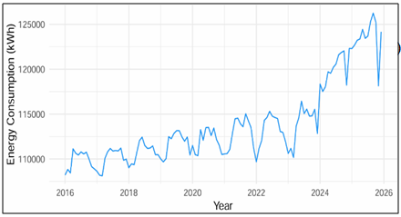
The study begins with an initial analysis of the dataset through a time series plot of the Monthly Electrical Energy Consumption of the Province of Nueva Vizcaya as shown in Figure 1. This section aims to visually assess the overall behavior and pattern of electrical energy consumption over the 120-month observation period, providing a preliminary understanding of trends and seasonality in the series.

Figure 1 presents the time series plot of monthly electrical energy consumption in the Province of Nueva Vizcaya from January 2016 to December 2025. Over the 120-month observation period, the series recorded a mean of 113,802 kWh (SD = 4,515.68 kWh), with values ranging from a minimum of 108,131 kWh to a maximum of 126,251 kWh. The median of 112,444 kWh falls below the mean, reflecting a right-skewed distribution consistent with the accelerating upward movement observed in the latter portion of the series, particularly from 2023 onward. Monthly consumption increased from an average of 109,822 kWh in 2016 to 123,527 kWh in 2025, representing an overall increase of approximately 11.1% over ten years. The standard deviation nearly doubled across the same period from 1,040 kWh to 2,044 kWh, indicating that consumption variability increased alongside the rising trend, a pattern commonly associated with growing electrification and economic expansion in developing provinces 3. In addition, stationarity tests confirm that the series is non-stationary. The ADF test with  indicating to accept the null hypothesis of a unit root at the 0.05 significance level 25, while the KPSS test rejected the null hypothesis of stationarity under both level and trend specifications, each with
  -values ≤ 0.01
 26. Together, both tests consistently confirm that the series is non-stationary and must be differenced prior to model fitting 17, 29.
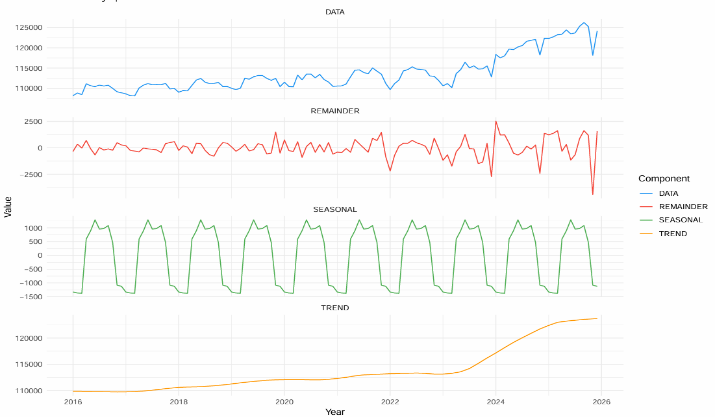
To examine the underlying structure of the series more thoroughly, STL decomposition was applied 27, as shown in Figure 2.

Figure 2 shows the STL decomposition of monthly electrical energy consumption in Nueva Vizcaya from 2016 to 2025, showing three main components. First, the trend indicates that electricity consumption remained relatively stable from 2016 to 2022, ranging between 110,000 and 113,000 kWh. However, it began to increase in 2023, reaching approximately 122,000 kWh by the end of 2025. This increase may be attributed to the growing number of electrified households and the economic recovery following the pandemic, a pattern commonly observed across developing provinces in the Philippines 3. Second, the seasonal component reveals a clear and consistent annual cycle throughout the entire period. Consumption tends to peak around the middle of the year during the dry season and at the beginning of the year. This climatically driven pattern has been well documented in studies on electricity demand in tropical regions 36, 37. The consistency of this seasonal pattern each year confirms that the additive decomposition method used is appropriate, as highlighted by 27. Third, the remainder component shows that the unexplained fluctuations in the data are minimal and appear random, with no discernible pattern. This is consistent with white noise, indicating that the analysis successfully captured the major features of the data 29. Overall, electricity consumption in the province exhibits a non-linear upward trend along with a stable and recurring seasonal pattern.
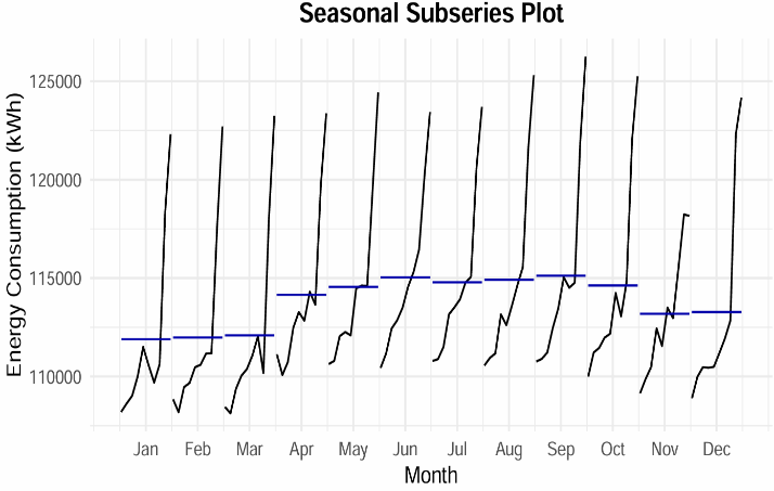
To further characterize the within-year seasonal structure of electrical energy consumption, a seasonal subseries plot was constructed as shown in Figure 3, following the approach described by Cleveland 38.
Figure 3 shows the Electrical Energy Consumption in Nueva Vizcaya for each month across all ten years, with a horizontal blue line showing the average for that month. The plot shows that consumption is lowest at the start of the year, with January and February averaging approximately 111,891 kWh and 111,980 kWh, respectively. It rises gradually through the middle months, remaining elevated from May through September, with September recording the highest monthly average at approximately 115,122 kWh, before declining slightly toward year-end. This mid-year peak is consistent with the dry season in the Philippines, during which higher ambient temperatures drive increased use of cooling appliances and irrigation systems 36. Importantly, the subseries plot also reveals a consistent upward shift across all twelve calendar months over the ten-year period, indicating that the overall growth in electricity demand is not confined to specific seasons but is distributed uniformly throughout the year 29.

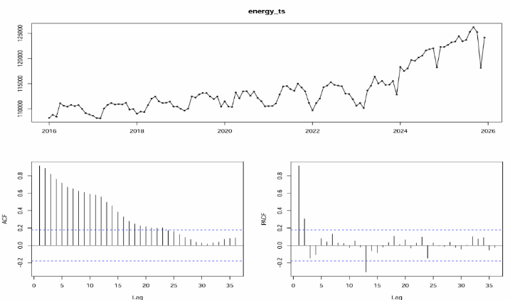
The ACF and PACF plots of the original series, shown in Figure 4, provide additional confirmation of non-stationarity.

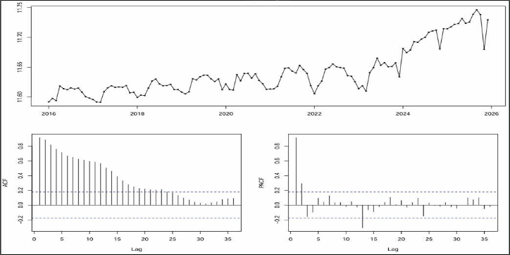
Figure 4 shows that the ACF exhibits a slow, gradual decay that remains statistically significant beyond lag 24, characteristic of a series with a non-stationary mean. The PACF shows a dominant spike at lag 1 that drops off sharply, suggesting that one regular difference is likely sufficient to remove the non-seasonal unit root 17. A notable spike at lag 13 in the PACF is consistent with the seasonal structure identified through STL decomposition, indicating the presence of a seasonal component that requires explicit treatment. Furthermore, the increasing spread of values observed in the time series plot suggests non-constant variance, pointing to the need for a log transformation prior to differencing 39. The log-transformed series and its ACF and PACF plots are presented in Figure 5.
Figure 5 shows that the transformed values range approximately from 11.58 to 11.75, and the spread of the data appears more uniform across time compared to the original series, confirming that the log transformation was effective in stabilizing the variance. However, the series retains a clear upward trend and the ACF continues to show slowly declining autocorrelations, confirming that the mean is still non-stationary and that differencing remains necessary. Figure 6 presents the results after applying one regular difference ( ) to the log-transformed series.


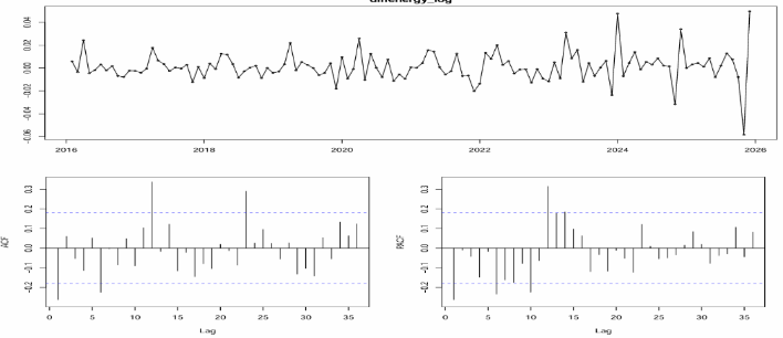
Figure 6 shows that the one regular differenced to the log-transformed electrical energy consumption in Nueva Vizcaya fluctuates around a mean of approximately zero within a narrow band of approximately  to
to , with no visible trend, indicating that the combination of log transformation and first-order differencing successfully removed the non-stationary behavior in the mean and variance 29. Most autocorrelations in both the ACF and PACF fall within the 95% confidence bounds. However, noticeable spikes remain at lag 12 in both plots, reaching approximately 0.30 in each, indicating that a yearly seasonal pattern persists after one regular difference. This finding confirmed that one seasonal difference at lag 12 (
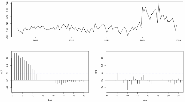
 ) as shown in Figure 7 was additionally required to fully remove the remaining seasonal non-stationarity before proceeding with model identification 17, 29.
Figure 7 shows the result after applying one seasonal difference ( ) at lag 12 to the log-transformed series. The time plot reveals that the series now fluctuates around a mean of approximately zero with no clear upward or downward trend, and the spread of values appears relatively stable throughout the observation period. The ACF and PACF plots further confirm that most autocorrelations have decayed within the 95% confidence bounds, with no dominant systematic spikes remaining. Together, the combination of log transformation, one regular difference (
 ), and one seasonal difference (
 ) was sufficient to achieve full stationarity in both the mean and variance of the series. With stationarity confirmed, the series is now ready for model identification, and the ACF and PACF plots will be used to guide the selection of appropriate ARIMA and SARIMA model orders 17, 29.

Following the confirmation of stationarity achieved through log transformation, one regular difference ( ), and one seasonal difference (
 ), a grid search was conducted in R to exhaustively evaluate all candidate
  and
and  model combinations as shown in Appendix A. Six competitive models were shortlisted for further evaluation, three ARIMA and SARIMA candidates, based on their AIC and BIC values, as summarized in Table 1.
Table 1 shows the identified top three ARIMA and SARIMA models, all three ARIMA candidates consistently recorded lower AIC and BIC values than all three SARIMA candidates. The difference between the best ARIMA model,  and the best SARIMA model,
 , exceeded 40 units in AIC and 35 units in BIC. A difference greater than 10 units constitutes very strong evidence in favor of the model with the lower value 40, making
  decisively superior to all SARIMA candidates on the basis of within-sample fit. Notably, even the third-ranked ARIMA model,
  with
with , still outperformed the best SARIMA model, further reinforcing the dominance of the non-seasonal ARIMA models in terms of in-sample fit criteria. Nevertheless, final model selection between the two top-performing candidates,
  and
and , was deferred to residual diagnostic checking and out-of-sample forecast accuracy evaluation on the January–December 2025 test set 29.
The two identified top-performing models were considered in this section,  from the non-seasonal model and
  from the seasonal model. These two models were selected for parameter estimation because they recorded the lowest AIC and BIC values within their respective models.
 . The estimated equation for the
  model, where
  represents the first-differenced series, is given by:
 | (9) |
The estimated autoregressive coefficients are ,
,  , and
, and  , while the moving average coefficients are
  and
and , with a constant
 . The term
  represents the white noise error term, assumed to equal zero for forecasting purposes.
 Since
Since  and
and , the model contains no autoregressive terms. Letting
  represents the doubly differenced series, the estimated model equation is:
 | (10) |
The non-seasonal moving average coefficient is , and the seasonal moving average coefficients are
  and
and  . No constant term was included in this model, as the total differencing order of
  makes the inclusion of a constant inadvisable 29.
Residual diagnostic checks were carried out for both models using the Ljung–Box test along with visual inspection of the residual time plot and ACF of the residuals. A model was considered adequate only if its residuals showed no significant autocorrelation, as indicated by a Ljung–Box  -value greater than 0.05 at lag 24 32.

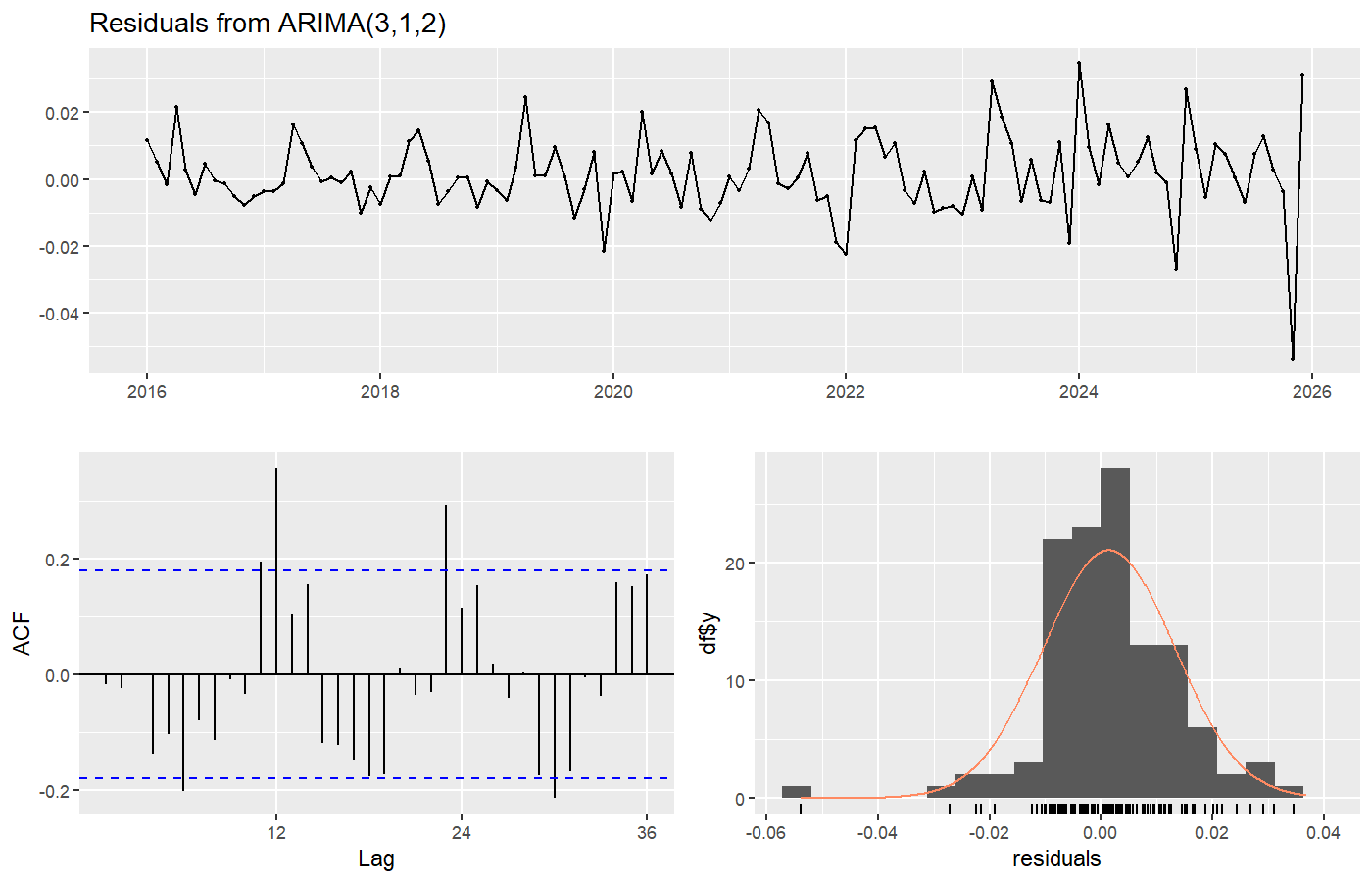
For  model, shown in Figure 8, the Ljung–Box test yielded a test statistic of
  with a
  -value of
  , below the 5% significance level. The null hypothesis of no residual autocorrelation was therefore rejected, with significant spikes observed in the residual ACF at lags 6, 11, 12, 23, and 30. Although the residual histogram displayed an approximately bell-shaped distribution centered near zero, normality alone is insufficient to declare model adequacy under the Box–Jenkins framework 17. Since the residuals remain autocorrelated,
  has not fully captured the systematic patterns in the series and is considered statistically inadequate for forecasting.

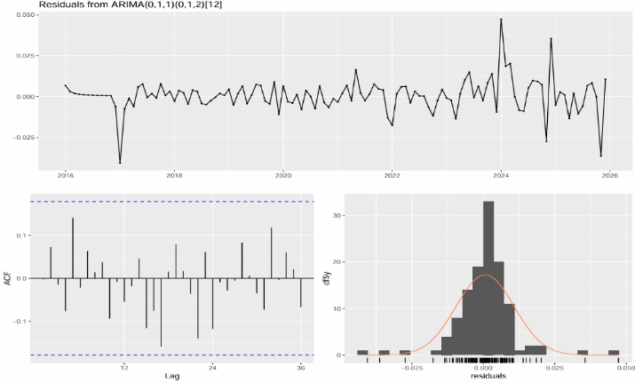
For  model, shown in Figure 9, the Ljung–Box test yielded
  with 21 degrees of freedom and a
  -value of 0.5367, well above the 5% threshold. The null hypothesis of no residual autocorrelation was therefore accepted. All bars in the residual ACF plot fell within the 95% confidence bounds, and the residual histogram showed an approximately normal distribution centered near zero.
  passed all diagnostic checks and was confirmed as a statistically adequate model, qualifying it for out-of-sample forecast accuracy evaluation on the 2025 test set.
Both models were refitted on the training set covering January 2016 to December 2024, and 12-month ahead forecasts were generated for the test period of January 2025 to December 2025. Forecast accuracy was evaluated using RMSE and MAPE. The results are summarized in Table 2.
As shown in Table 2, while  recorded lower in-sample fit values with
  and
and  compared to
  with
with  and
and  , it failed the residual diagnostic check due to significant autocorrelation remaining in its residuals. A model with autocorrelated residuals has not fully captured the structure of the data and cannot be considered reliable for forecasting under the Box–Jenkins framework, regardless of its in-sample fit (Box et al., 2015).
  on the other hand, passed all residual diagnostic checks and also achieved superior out-of-sample forecast accuracy, recording lower RMSE (0.01014) and MAPE (0.0555) values than
  . This indicates that
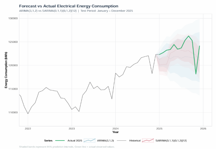
  not only fits the data adequately but also generalizes better to unseen observations. Figure 10 provides a visual confirmation of these findings.

Figure 10 shows that the SARIMA model tracks the actual 2025 consumption values, ranging from approximately 118,000 to 126,000 kWh more closely than the ARIMA model, whose forecasts remain relatively flat and fail to capture the seasonal fluctuations present in the actual series. Based on the combined evidence from diagnostic checking and out-of-sample forecast accuracy as shown in Table 2,  was selected as the best-fitting model for forecasting monthly electrical energy consumption in the Province of Nueva Vizcaya, Philippines.

The selected  model was refitted on the full dataset spanning January 2016 to December 2025 and used to generate monthly forecasts for January to December 2026. The fitted model is expressed as the equation (10):
 |
where  represents the doubly differenced log-transformed series, with
  represents the non-seasonal trend and
  represents the seasonal component at lag 12. The non-seasonal moving average coefficient is
 , and the seasonal moving average coefficients are
  and
and . The term
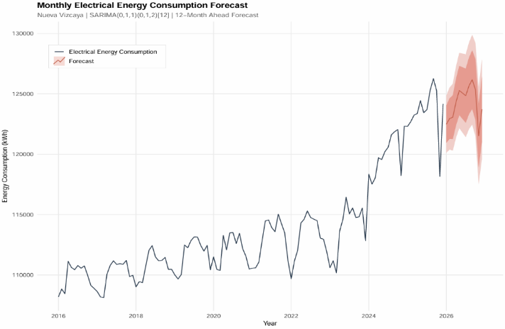
  denotes the white noise error term, assumed to equal zero for forecasting purposes. The forecast results, along with their 95% prediction intervals, are presented in Table 3 and visualized in Figure 11.
Table 3 presents the forecasted monthly electrical energy consumption in the province of Nueva Vizcaya using the best-fitting model  from January to December 2026 that ranges from a low of 121,527.40 kWh in November to a peak of 126,178.50 kWh in September, with a secondary low of 122,492.60 kWh in January. This within-year pattern, with lower values at the start and end of the year and higher values concentrated in the mid-year months is consistent with the seasonal structure identified throughout the analysis, reflecting the influence of the dry season and its associated increase in cooling and irrigation-related electricity demand 36. The overall level of the forecasted values, all exceeding 121,000 kWh per month, is higher than most months recorded before 2024, confirming that the province's electricity demand continues on an upward trajectory.

Figure 11 shows that the 95% prediction intervals (light shaded region) widen progressively as the forecast horizon extends further into 2026, reflecting the natural increase in uncertainty associated with longer-range forecasting. The interval width for January 2026 is approximately 2,712.60 kWh, while that for December 2026 is approximately 8,204.80 kWh, a pattern consistent with the behavior of well-specified SARIMA models 29. These forecasted values and their associated confidence bounds offer actionable, data-driven projections that energy planners and local government officials in Nueva Vizcaya can use to prepare for future electricity demand, support budget planning for energy expenditure, and inform the province's ongoing transition toward renewable energy sources.
This study forecasted the monthly electrical energy consumption of the Province of Nueva Vizcaya from January 2016 to December 2025 using ARIMA and SARIMA models developed through the Box–Jenkins methodology, covering all eight consumer sectors with an average monthly consumption of 113,802 kWh. The behavioral analysis revealed a clear upward trend of approximately 11.1% over ten years from 109,822 kWh in 2016 to 123,527 kWh in 2025, alongside a stable seasonal pattern peaking between May and September during the dry season. The comparative model evaluation showed that although  recorded lower AIC (−701.44) and BIC (−684.76), it failed the residual diagnostic check due to significant autocorrelation in its residuals, rendering it statistically inadequate for forecasting.
  by contrast, passed all diagnostic checks with a Ljung–Box p-value of 0.5367 and achieved superior out-of-sample accuracy with lower RMSE (0.01014) and MAPE (0.0555) on the 2025 test set, confirming it as the best-fitting model. The 2026 forecasts, projecting monthly consumption between 121,527.40 kWh and 126,178.50 kWh, reflect the province's sustained upward demand trajectory and provide reliable, data-driven projections that directly support the province's progress toward SDG 7 (Affordable and Clean Energy). These forecasts enable NUVELCO and the local government to plan energy supply more efficiently, manage the PHP 43 million annual electricity budget more effectively, and direct resources toward extending electricity access to remaining unelectrified sitio-level communities in remote municipalities, a goal that serves as a foundational prerequisite for advancing SDG 1 (No Poverty), SDG 3 (Good Health and Well-Being), SDG 4 (Quality Education), and SDG 8 (Decent Work and Economic Growth). Furthermore, the seasonal demand pattern captured by the model can guide load distribution and maintenance scheduling during high-demand periods, while the forecast baseline supports the province's ongoing renewable energy transition, simultaneously advancing SDG 7 and SDG 13 (Climate Action) by reducing dependence on fossil fuel-based generation 3, 6.
Based on the findings of this study, several recommendations are offered. NUVELCO and the Provincial Government of Nueva Vizcaya are encouraged to adopt  as a practical short-term demand planning tool, updated regularly as new data become available, to support evidence-based energy supply management aligned with SDG 7. Future studies should explore the incorporation of exogenous variables, such as temperature, population, tariff rates, and economic indicators, through ARIMAX or SARIMAX frameworks to improve model responsiveness to climate variability and strengthen alignment with SDG 13. Future research should further compare SARIMA against machine learning and hybrid approaches such as Long Short-Term Memory (LSTM), Extreme Gradient Boosting (XGBoost), Random Forest, and ARIMA-LSTM to determine whether more flexible models can offer additional forecast accuracy gains over longer horizons. The demand projections produced in this study should also guide the planning and sizing of renewable energy installations in the province, directly advancing SDG 7 and SDG 13 at the subnational level. Finally, the methodological framework applied in this study is recommended as a replicable template for province-level electricity forecasting across other regions of the Philippines, contributing to a more systematic and evidence-based approach to subnational energy planning.
The author sincerely expresses deep gratitude to the Department of Science and Technology-Science Education Institute (DOST-SEI) through the Capacity Building Program in Science and Mathematics Education (CBPSME), for their steadfast support and guidance throughout the development of this paper. Their continued encouragement and assistance played a vital role in the successful completion of this research endeavor.
| [1] | Samuel, J. (2022). Forecasting electricity consumption in the Philippines using ARIMA models. International Journal of Machine Learning and Computing, 12(6). | ||
| In article | View Article | ||
| [2] | Urrutia, J. D., Resurreccion, N. C., Visco, L. M. C., Bautista, L. A., Malvar, R. J., Oliquino, A. B., & Gano, L. A. (2018). Daily prediction of electricity rates of distribution utilities in Luzon. Indian Journal of Science and Technology, 11(20), 1–8. | ||
| In article | View Article | ||
| [3] | International Energy Agency. (2023). World energy outlook 2023. IEA. https://www.iea.org/reports/world-energy-outlook-2023. | ||
| In article | View Article | ||
| [4] | International Energy Agency. (2020). Global energy review 2020: The impacts of the Covid-19 crisis on global energy demand and CO₂ emissions. IEA. https://www.iea.org/reports/global-energy-review-2020. | ||
| In article | View Article | ||
| [5] | Department of Energy. (2020). Philippine energy situation: 2020 annual report. DOE. https://www.doe.gov.ph. | ||
| In article | |||
| [6] | United Nations. (2015). Transforming our world: The 2030 agenda for sustainable development. United Nations. https://sdgs.un.org/2030agenda. | ||
| In article | |||
| [7] | Torculas, E., Rentillo, E. J., & Ambita, A. A. (2023). Forecasting of energy consumption in the Philippines using machine learning algorithms. In Communications in computer and information science (pp. 424–435). | ||
| In article | View Article | ||
| [8] | Ortigoza-Larroza, C., Rivas-Martínez, G. I., Grillo, S., & Benítez, E. (2025). Residential Electricity Consumption Forecasting using Machine Learning and SARIMA Approaches: A Case Study of Paraguay. International Journal of Energy and Water Resources, 10(1). | ||
| In article | View Article | ||
| [9] | Ramos, P. V. B., Villela, S. M., Silva, W. N., & Dias, B. H. (2023). Residential energy consumption forecasting using deep learning models. Applied Energy, 350, 121705. | ||
| In article | View Article | ||
| [10] | Nazir, A., Shaikh, A. K., Shah, A. S., & Khalil, A. (2023). Forecasting energy consumption demand of customers in smart grid using Temporal Fusion Transformer (TFT). Results in Engineering, 17, 100888. | ||
| In article | View Article | ||
| [11] | Amalou, I., Mouhni, N., & Abdali, A. (2022). Multivariate time series prediction by RNN architectures for energy consumption forecasting. Energy Reports, 8, 1084–1091. | ||
| In article | View Article | ||
| [12] | Pierre, A. A., Akim, S. A., Semenyo, A. K., & Babiga, B. (2023). Peak Electrical Energy Consumption Prediction by ARIMA, LSTM, GRU, ARIMA-LSTM and ARIMA-GRU approaches. Energies, 16(12), 4739. | ||
| In article | View Article | ||
| [13] | Klyuev, R. V., Morgoev, I. D., Morgoeva, A. D., Gavrina, O. A., Martyushev, N. V., Efremenkov, E. A., & Mengxu, Q. (2022). Methods of Forecasting Electric Energy Consumption: A Literature review. Energies, 15(23), 8919. | ||
| In article | View Article | ||
| [14] | Jalambo, M., Saquin, P. L., Dalis, I., Saumat, M., Rupinta, M., & Demecillo, G. (2025). Analysis and forecasting of electricity demand in MOELCI-II using ARIMA Model. International Journal for Multidisciplinary Research, 7(4). | ||
| In article | View Article | ||
| [15] | Arumugam, V., & Natarajan, V. (2023). Time series modeling and forecasting using autoregressive integrated moving average and seasonal autoregressive integrated moving average models. Instrumentation Mesure Métrologie, 22(4), 161–168. | ||
| In article | View Article | ||
| [16] | Hossain, M. L., Shams, S. M. N., & Ullah, S. M. (2025). Time-series and deep learning approaches for renewable energy forecasting in Dhaka: a comparative study of ARIMA, SARIMA, and LSTM models. Discover Sustainability, 6(1). | ||
| In article | View Article | ||
| [17] | Box, G.E., Jenkins, G.M., Reinsel, G.C. and Ljung, G.M. (2015) Time Series Analysis: Forecasting and Control. John Wiley & Sons, Hoboken. | ||
| In article | |||
| [18] | Delima, A. J. P. (2019). Application of time series analysis in projecting Philippines’ electric consumption. International Journal of Machine Learning and Computing, 9(5), 694–699. | ||
| In article | View Article | ||
| [19] | Parreno, S. J. (2023). Forecasting the total non-coincidental monthly system peak demand in the Philippines: a comparison of seasonal autoregressive integrated moving average models and artificial neural networks. International Journal of Energy Economics and Policy, 13(5), 544–552. | ||
| In article | View Article | ||
| [20] | Domingo, C. J. (2024). Electrical energy consumption models in the province of Nueva Vizcaya (Unpublished thesis). | ||
| In article | |||
| [21] | Tolentino, J. A. (2025). Forecasting electricity consumption using ARIMA model. In Lecture notes in networks and systems (pp. 41–51). | ||
| In article | View Article | ||
| [22] | Mahusay, A. T., & Fenomeno, S. D. (2022). Electricity Consumption Prediction Model for Southern Luzon State University-Main Campus using Artificial Neural Network. 2022 IEEE 12th Annual Computing and Communication Workshop and Conference (CCWC), 3, 0038–0044. | ||
| In article | View Article | ||
| [23] | Nueva Vizcaya, Philippines. (2025). Physiological features and natural Resources - Nueva Vizcaya, Philippines. Nueva Vizcaya, Philippines - Naturally Vibrant and Watershed Haven of the Cagayan Valley. https://nuevavizcaya.gov.ph/physiological-features-and-natural-resources/. | ||
| In article | |||
| [24] | Philippine Statistics Authority. (2020). 2020 census of population and housing: Nueva Vizcaya provincial profile. PSA. https://www.psa.gov.ph. | ||
| In article | |||
| [25] | Dickey, D. A., & Fuller, W. A. (1979). Distribution of the Estimators for Autoregressive Time Series with a Unit Root. Journal of the American Statistical Association, 74(366a), 427–431. | ||
| In article | View Article | ||
| [26] | Kwiatkowski, D., Phillips, P.C.B., Schmidt, P. and Shin, Y. (1992) Testing the Null Hypothesis of Stationarity against the Alternative of a Unit Root. Journal of Econometrics, 54, 159-178. | ||
| In article | View Article | ||
| [27] | Cleveland, R.B., Cleveland, W.S., McRae, J.E., & Terpenning, I. (1990). STL: A seasonal-trend decomposition procedure based on Loess. Journal of Official Statistics, 6(1), 3–73. | ||
| In article | |||
| [28] | Box, G. E. P., & Cox, D. R. (1964). An analysis of transformations. Journal of the Royal Statistical Society Series B (Statistical Methodology), 26(2), 211–243. | ||
| In article | View Article | ||
| [29] | Hyndman, R. J., & Athanasopoulos, G. (2021). Forecasting: Principles and Practice (3rd ed.). OTexts. https://otexts.com/fpp3/. | ||
| In article | |||
| [30] | Hyndman, R.J., Athanasopoulos, G., Bergmeir, C., Caceres, G., Chhay, L., O'Hara-Wild, M., Petropoulos, F., Razbash, S., Wang, E., & Yasmeen, F. (2023). forecast: Forecasting functions for time series and linear models. R package version 8.21. https://pkg.robjhyndman.com/forecast/. | ||
| In article | View Article | ||
| [31] | Hyndman, R.J. and Khandakar, Y. (2008) Automatic Time Series Forecasting: The Forecast Package for R. Journal of Statistical Software, 27(3), 1-22. | ||
| In article | View Article | ||
| [32] | Ljung, G.M. and Box, G.E.P. (1978) On a Measure of a Lack of Fit in Time Series Models. Biometrika, 65(2), 297-303. | ||
| In article | View Article | ||
| [33] | Akaike, H. (1974). A new look at the statistical model identification. IEEE Transactions on Automatic Control, 19(6), 716–723. | ||
| In article | View Article | ||
| [34] | Schwarz, G. (1978) Estimating the Dimension of a Model. Annals of Statistics, 6(2), 461-464. | ||
| In article | View Article | ||
| [35] | Makridakis, S. (1993). Accuracy measures: theoretical and practical concerns. International Journal of Forecasting, 9(4), 527–529. | ||
| In article | View Article | ||
| [36] | Sailor, D., & Muñoz, J. R. (1997). Sensitivity of electricity and natural gas consumption to climate in the U.S.A.—Methodology and results for eight states. Energy, 22(10), 987–998. | ||
| In article | View Article | ||
| [37] | Moral-Carcedo, J., & Vicéns-Otero, J. (2005). Modelling the non-linear response of Spanish electricity demand to temperature variations. Energy Economics, 27(3), 477–494. | ||
| In article | View Article | ||
| [38] | Cleveland, W.S. (1993) Visualizing Data. Hobart Press, Summit. | ||
| In article | |||
| [39] | Wei, W.W.S. (2006). Time Series Analysis, Univariate and Multivariate Methods. 2nd Edition, Pearson Addision Wesley, New York. | ||
| In article | |||
| [40] | Burnham, K.P. and Anderson, D.R. (2002) Model Selection and Inference: A Practical Information-Theoretic Approach. 2nd Edition, Springer-Verlag, New York. | ||
| In article | |||
Published with license by Science and Education Publishing, Copyright © 2026 Alberto M. Camangian
 This work is licensed under a Creative Commons Attribution 4.0 International License. To view a copy of this license, visit
http://creativecommons.org/licenses/by/4.0/
This work is licensed under a Creative Commons Attribution 4.0 International License. To view a copy of this license, visit
http://creativecommons.org/licenses/by/4.0/
| [1] | Samuel, J. (2022). Forecasting electricity consumption in the Philippines using ARIMA models. International Journal of Machine Learning and Computing, 12(6). | ||
| In article | View Article | ||
| [2] | Urrutia, J. D., Resurreccion, N. C., Visco, L. M. C., Bautista, L. A., Malvar, R. J., Oliquino, A. B., & Gano, L. A. (2018). Daily prediction of electricity rates of distribution utilities in Luzon. Indian Journal of Science and Technology, 11(20), 1–8. | ||
| In article | View Article | ||
| [3] | International Energy Agency. (2023). World energy outlook 2023. IEA. https://www.iea.org/reports/world-energy-outlook-2023. | ||
| In article | View Article | ||
| [4] | International Energy Agency. (2020). Global energy review 2020: The impacts of the Covid-19 crisis on global energy demand and CO₂ emissions. IEA. https://www.iea.org/reports/global-energy-review-2020. | ||
| In article | View Article | ||
| [5] | Department of Energy. (2020). Philippine energy situation: 2020 annual report. DOE. https://www.doe.gov.ph. | ||
| In article | |||
| [6] | United Nations. (2015). Transforming our world: The 2030 agenda for sustainable development. United Nations. https://sdgs.un.org/2030agenda. | ||
| In article | |||
| [7] | Torculas, E., Rentillo, E. J., & Ambita, A. A. (2023). Forecasting of energy consumption in the Philippines using machine learning algorithms. In Communications in computer and information science (pp. 424–435). | ||
| In article | View Article | ||
| [8] | Ortigoza-Larroza, C., Rivas-Martínez, G. I., Grillo, S., & Benítez, E. (2025). Residential Electricity Consumption Forecasting using Machine Learning and SARIMA Approaches: A Case Study of Paraguay. International Journal of Energy and Water Resources, 10(1). | ||
| In article | View Article | ||
| [9] | Ramos, P. V. B., Villela, S. M., Silva, W. N., & Dias, B. H. (2023). Residential energy consumption forecasting using deep learning models. Applied Energy, 350, 121705. | ||
| In article | View Article | ||
| [10] | Nazir, A., Shaikh, A. K., Shah, A. S., & Khalil, A. (2023). Forecasting energy consumption demand of customers in smart grid using Temporal Fusion Transformer (TFT). Results in Engineering, 17, 100888. | ||
| In article | View Article | ||
| [11] | Amalou, I., Mouhni, N., & Abdali, A. (2022). Multivariate time series prediction by RNN architectures for energy consumption forecasting. Energy Reports, 8, 1084–1091. | ||
| In article | View Article | ||
| [12] | Pierre, A. A., Akim, S. A., Semenyo, A. K., & Babiga, B. (2023). Peak Electrical Energy Consumption Prediction by ARIMA, LSTM, GRU, ARIMA-LSTM and ARIMA-GRU approaches. Energies, 16(12), 4739. | ||
| In article | View Article | ||
| [13] | Klyuev, R. V., Morgoev, I. D., Morgoeva, A. D., Gavrina, O. A., Martyushev, N. V., Efremenkov, E. A., & Mengxu, Q. (2022). Methods of Forecasting Electric Energy Consumption: A Literature review. Energies, 15(23), 8919. | ||
| In article | View Article | ||
| [14] | Jalambo, M., Saquin, P. L., Dalis, I., Saumat, M., Rupinta, M., & Demecillo, G. (2025). Analysis and forecasting of electricity demand in MOELCI-II using ARIMA Model. International Journal for Multidisciplinary Research, 7(4). | ||
| In article | View Article | ||
| [15] | Arumugam, V., & Natarajan, V. (2023). Time series modeling and forecasting using autoregressive integrated moving average and seasonal autoregressive integrated moving average models. Instrumentation Mesure Métrologie, 22(4), 161–168. | ||
| In article | View Article | ||
| [16] | Hossain, M. L., Shams, S. M. N., & Ullah, S. M. (2025). Time-series and deep learning approaches for renewable energy forecasting in Dhaka: a comparative study of ARIMA, SARIMA, and LSTM models. Discover Sustainability, 6(1). | ||
| In article | View Article | ||
| [17] | Box, G.E., Jenkins, G.M., Reinsel, G.C. and Ljung, G.M. (2015) Time Series Analysis: Forecasting and Control. John Wiley & Sons, Hoboken. | ||
| In article | |||
| [18] | Delima, A. J. P. (2019). Application of time series analysis in projecting Philippines’ electric consumption. International Journal of Machine Learning and Computing, 9(5), 694–699. | ||
| In article | View Article | ||
| [19] | Parreno, S. J. (2023). Forecasting the total non-coincidental monthly system peak demand in the Philippines: a comparison of seasonal autoregressive integrated moving average models and artificial neural networks. International Journal of Energy Economics and Policy, 13(5), 544–552. | ||
| In article | View Article | ||
| [20] | Domingo, C. J. (2024). Electrical energy consumption models in the province of Nueva Vizcaya (Unpublished thesis). | ||
| In article | |||
| [21] | Tolentino, J. A. (2025). Forecasting electricity consumption using ARIMA model. In Lecture notes in networks and systems (pp. 41–51). | ||
| In article | View Article | ||
| [22] | Mahusay, A. T., & Fenomeno, S. D. (2022). Electricity Consumption Prediction Model for Southern Luzon State University-Main Campus using Artificial Neural Network. 2022 IEEE 12th Annual Computing and Communication Workshop and Conference (CCWC), 3, 0038–0044. | ||
| In article | View Article | ||
| [23] | Nueva Vizcaya, Philippines. (2025). Physiological features and natural Resources - Nueva Vizcaya, Philippines. Nueva Vizcaya, Philippines - Naturally Vibrant and Watershed Haven of the Cagayan Valley. https://nuevavizcaya.gov.ph/physiological-features-and-natural-resources/. | ||
| In article | |||
| [24] | Philippine Statistics Authority. (2020). 2020 census of population and housing: Nueva Vizcaya provincial profile. PSA. https://www.psa.gov.ph. | ||
| In article | |||
| [25] | Dickey, D. A., & Fuller, W. A. (1979). Distribution of the Estimators for Autoregressive Time Series with a Unit Root. Journal of the American Statistical Association, 74(366a), 427–431. | ||
| In article | View Article | ||
| [26] | Kwiatkowski, D., Phillips, P.C.B., Schmidt, P. and Shin, Y. (1992) Testing the Null Hypothesis of Stationarity against the Alternative of a Unit Root. Journal of Econometrics, 54, 159-178. | ||
| In article | View Article | ||
| [27] | Cleveland, R.B., Cleveland, W.S., McRae, J.E., & Terpenning, I. (1990). STL: A seasonal-trend decomposition procedure based on Loess. Journal of Official Statistics, 6(1), 3–73. | ||
| In article | |||
| [28] | Box, G. E. P., & Cox, D. R. (1964). An analysis of transformations. Journal of the Royal Statistical Society Series B (Statistical Methodology), 26(2), 211–243. | ||
| In article | View Article | ||
| [29] | Hyndman, R. J., & Athanasopoulos, G. (2021). Forecasting: Principles and Practice (3rd ed.). OTexts. https://otexts.com/fpp3/. | ||
| In article | |||
| [30] | Hyndman, R.J., Athanasopoulos, G., Bergmeir, C., Caceres, G., Chhay, L., O'Hara-Wild, M., Petropoulos, F., Razbash, S., Wang, E., & Yasmeen, F. (2023). forecast: Forecasting functions for time series and linear models. R package version 8.21. https://pkg.robjhyndman.com/forecast/. | ||
| In article | View Article | ||
| [31] | Hyndman, R.J. and Khandakar, Y. (2008) Automatic Time Series Forecasting: The Forecast Package for R. Journal of Statistical Software, 27(3), 1-22. | ||
| In article | View Article | ||
| [32] | Ljung, G.M. and Box, G.E.P. (1978) On a Measure of a Lack of Fit in Time Series Models. Biometrika, 65(2), 297-303. | ||
| In article | View Article | ||
| [33] | Akaike, H. (1974). A new look at the statistical model identification. IEEE Transactions on Automatic Control, 19(6), 716–723. | ||
| In article | View Article | ||
| [34] | Schwarz, G. (1978) Estimating the Dimension of a Model. Annals of Statistics, 6(2), 461-464. | ||
| In article | View Article | ||
| [35] | Makridakis, S. (1993). Accuracy measures: theoretical and practical concerns. International Journal of Forecasting, 9(4), 527–529. | ||
| In article | View Article | ||
| [36] | Sailor, D., & Muñoz, J. R. (1997). Sensitivity of electricity and natural gas consumption to climate in the U.S.A.—Methodology and results for eight states. Energy, 22(10), 987–998. | ||
| In article | View Article | ||
| [37] | Moral-Carcedo, J., & Vicéns-Otero, J. (2005). Modelling the non-linear response of Spanish electricity demand to temperature variations. Energy Economics, 27(3), 477–494. | ||
| In article | View Article | ||
| [38] | Cleveland, W.S. (1993) Visualizing Data. Hobart Press, Summit. | ||
| In article | |||
| [39] | Wei, W.W.S. (2006). Time Series Analysis, Univariate and Multivariate Methods. 2nd Edition, Pearson Addision Wesley, New York. | ||
| In article | |||
| [40] | Burnham, K.P. and Anderson, D.R. (2002) Model Selection and Inference: A Practical Information-Theoretic Approach. 2nd Edition, Springer-Verlag, New York. | ||
| In article | |||