1. Introduction

Every research is characterised by a population, which is the entire group of people or objects, described by some characteristics, on which the researcher collects data ^{[1, 2]}. Ultimately, the researcher would have to collect data on every person or object in the population to maximise the chance of reaching results that represent the population characteristics of interest. Unfortunately research conditions, such as unavailability of resources (e.g. time and funds) to collect data on the entire population, often compels researchers to resort to collecting data on a subset of the population often called a sample.

Researchers have the freedom to use a sample instead of the entire population under the condition that they will be able to use the sample to reach results, called sample statistics, which exactly or closely represent the population characteristics of interest, generally referred to as parameters. The degree to which a sample statistic is equal to its parameter is termed precision ^{[2, 3]}. Every researcher expects a high precision or a situation where the resulting statistics are equal or almost equal to their parameters.

The best way to ensure that the use of a sample leads to precise results or an estimation of the parameter of interest is to make the sample representative ^{[4, 5]}. A representative sample could be said to be a subset of the population which is large enough to lead to an estimation of the parameters of interest. Representative samples are more likely to yield results or statistics that at least approximate the parameters of interest.

A strong consensus exists among researchers [1-7]^[1] regarding the idea that a sample’s representativeness improves as its size gets closer to the population size. Invariably the larger the sample, the higher the chance of the resulting statistics approximating population parameters, all other factors held constant. The statement “the larger the sample, the better” has therefore become a maxim among researchers, especially quantitative and objectivist researchers. Consequently many researchers and writers ^{[1, 7]} have expended efforts to produce formulae and tables for determining representative sample sizes in research.

Krejcie and Morgan ^[7] generated one of the earliest sample size determination tables and formulae. Their table was operationalized based on the principle behind the maxim earlier mentioned. Bartlett et al. ^[7], Eng ^[6], and other researchers were also motivated by this principle to generate sample size determination tables and formulae. A research work by Hanley and Moodie ^[3] indicates that efforts to determine these formulae and tables have been primarily fuelled by sampling theory, including the Law of Large Numbers (LLN) and related theories. As a result, the idea that larger samples better support estimation of population parameters is more theoretical and less empirical.

While the foregoing school of thought is not necessarily unimportant, its existence is mocked by the absence of empirical evidences on it. It is logical to say that credibility and acceptability of the several sample size formulae and tables developed over the years are weak without empirical evidence to the idea of larger samples better supporting estimation of parameters. It is worth revealing that researchers like Brown ^[2] and Fiske et al. ^[8] have tried to empirically demonstrate the effect of sample size on how well statistics approximate parameters. Yet we think their contributions, including those of other researchers, are not sufficient to back the vehemence with which researchers and people in the academic world apply the idea of higher samples better supporting estimation of population parameters. Our argument is based on these observations:

(1) None of these researchers has been able to produce empirical evidence using all the statistics associated with statistical estimation. In other words, these researchers focused on one type of statistic or a limited number of statistics. For instance, Brown ^[2] focused on the effect of sample size on standard error of the mean (SEM) which is a measure of precision, whereas Springate ^[5] focused on the effect of sample size on the reliability of estimates of error. We are however of the view that the mean and median and their associated standard deviation (SD) are in almost all cases the basic parameters of interest in statistical estimation, whereas confidence interval (CI) and SEM are supporting statistics and indicators of statistical precision. Therefore the relationship between sample size and each of: (a) the sample mean and its SD and SEM; and (b) Median and its SD and SEM, is deemed better empirical evidence on whether or not larger samples support estimation of population parameters.

(2) Some statistical treatments that we think should have been used to provide evidences on the relationship between sample size and statistical precision have not been applied by these researchers. One way to produce this evidence is to relate a distribution of varying sample sizes to their corresponding probability values (i.e. p-values) in terms of a one-sample t-test that tests the difference between a mean statistic and its population parameter. In this case, the p-value gets larger than its theoretical value as the sample mean better approximates the population parameter.

In this paper therefore, we tried to know if the use of larger samples really lead to statistics that better approximate parameters by assessing the correlation between sample size and the sample mean and median, and their respective SD, SEM and CI. We focused on the mean and median because statistical estimation and inference is largely based on them. It is hoped that this study will contribute to knowledge on whether or not larger samples support estimation of population parameters by using a more robust technique. We also attempted to provide the empirical rationale for using representative samples by quantitative researchers.

Statistical inference is one of the most commonly used terms among researchers. This situation is however not an oddity because statistical inference is the essence of all quantitative researches. The term, often also used as Inferential Statistics, is the process of deducing properties of an underlying population or distribution by analysis of data ^{[9, 10]}. The properties of interest are the population characteristics one wants to deduce such mean, median and standard deviation. In statistical inference, the researcher infers characteristics about a population through statistical estimation or/and hypotheses testing. This paper focuses on statistical estimation, which is the basis of statistical inference.

Statistical estimation is basically the process of deducing the property of a distribution or population using some data [^[9], p. 375]. There are two main forms of statistical estimation. Point estimation is one of the main forms of statistical estimation concerned with deducing a precise or particular value that best approximates a population parameter of interest [^[10], p. 99]. For example, the average salary of the population of employees in a company is 566.90 USD, a value which is a point estimate. An interval estimate is an interval developed using a dataset drawn from a population so that under repeated sampling of these datasets the interval would contain the true parameter based on the probability representing the confidence level ^{[9, 10]}. With reference to the first cited example, the average salary of the population of employees in the company falls in the interval of values from 456.21 USD to 643.32 USD.

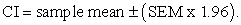
Confidence intervals are constructed based primarily on a level of confidence, which is the percentage of all possible samples that can be expected to include the true population parameter [^[11], p. 153]. The most commonly used confidence level is 95%, though 99% and other levels could be used. A confidence interval could be mathematically expressed as:

(1)

In equation 1, SEM is the standard error of the mean and 1.96 is the 0.975 quintile of the normal distribution. The CI is even more important from the point of view of its lower and upper limits. With respect to equation 1, the lower limit is given as:

(2)

The upper limit is given by:

(3)

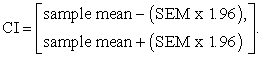
The confidence interval represented by equation 1 is therefore given by:

(4)

In the above equations, SEM is the standard deviation of the sampling distribution of the sample mean. It is generally used as a measure of the precision of an estimate, and its size affects the confidence interval ^{[2, 10]}. Apart from its influence on the confidence interval, SEM is often considered alongside the sample statistic to known how well the statistic approximates the population parameter. As a result, SEM is a basic indicator of whether or not a point or interval estimate approximates the population mean well. It is worth noting that the standard error of the mean could be based on other statistics, not only the mean.

The SEM is mathematically linked to the sample standard deviation (an estimator of the variability in the population) and sample size, assuming statistical independence of the values in the sample. The mathematical relationship is expressed as:

(5)

The sample mean is also mathematically expressed as:

(6)

The population mean the sample mean is expected to approximate is given by:

(7)

In equations 5, x_i stands for the distribution of sample observations and n stands for the number of sample observations, or sample size. The true population mean is represented by equation 7. With respect to equation 7, X_i stands for the distribution of population observations and N stands for the number of population observations, or population size. Moreover in equations 5 and 6, the sample size, n, makes a major influence on SEM and sample mean. Equation 5 therefore reflects the dependence of interval estimates on sample size, whereas equation 6 reveals the influence of sample size on a point estimate, which is the sample mean. For normally distributed data, the mean approximate the median ^{[1, 11]}. Therefore, sample size influences the sample median as much as its influences the sample mean for normally distributed data.

Another important statistical component of an interval estimate is the sample standard deviation, s, which is related to SEM and n in equation 5. The standard deviation is theoretically a measure of the spread of data from the mean. The LLN suggests that the standard deviation of sampled dataset gets closer to the population standard deviation as the sample size increases. Probability theory also suggests that there is a higher likelihood of the sample statistic approximating the population parameter as the sample randomly drawn from the population increases in size. Thus the larger the sample size relative to the population size, the higher the probability of the sample statistic approximating the population parameter of interest. On the basis of this theory and the LLN, it could additionally be said that the estimation of all population parameters yields more precise results as sample size increases.

Some researchers ^{[2, 8]} have confirmed a positive correlation between sample size and statistical precision in terms of SEM. Some have also observed empirically that sample size is correlated (negatively) to statistical power. In this paper, we enhance the scope of the empirical evidence by testing the correlation between sample size and each of all the basic statistics associated with statistical estimation, namely the mean and median and their respective SD, SEM and CI. Since the mean is equal to the median for normal distributions and all distributions simulated in this study are normal distributions (See Table 8), we do not directly include the median and its SD, SEM and CI. We hypothesize that the larger the sample drawn randomly from a population, the better the sample statistic approximates the population parameter.

Let us assume that a researcher’s interest is to use a sample to estimate the population mean (which we represent with X) of a normal distribution. The mean statistic obtained is represented as x. In statistical estimation, the researcher expects that X = x, or x approximates X so that he can infer to the population. The researcher can conduct a statistical test for a difference between X and x and make a decision regarding the difference between them based on the resulting probability value (i.e. p-value or significance level). In probability theory, the probability value is the probability of getting a result (such as a mean statistic) equal to or more extreme than what was actually observed, assuming that the hypothesis under consideration is true [^[12], p. 886]. The rule of thumb is that the p-value, which is based on the observed data, must be greater than the level of significance (α), the theoretical p-value, if x = X, or if x approximates X. Therefore the closer x is to X, the more the calculated p-value becomes greater than the theoretical significance level, which is often 95%. In view of our hypothesis, we expect that the calculated significance level increases as sample size increases. Invariably, x gets more equal to X with increasing sample size so that the p-value increases towards the maximum possible value. In this paper therefore, we demonstrate the robustness of our statistical treatments by examining the extent to which the calculated p-value changes with increasing sample size relative to the theoretical p-value. The research methodology adopted is explained in the next section.

2. Materials and Methods

We used simulation to generate data that met all necessary conditions, namely: (a) normality of each drawn sample; (b) randomness of all samples; and (c) exhaustiveness of the population, which means that several samples of different sizes were drawn from the population so that the distribution of sample sizes spanned the lower, middle and upper sections of the distribution of the population items. Each of these conditions is of special importance. Normality of each simulated sample made way for equating the mean to the median. Randomness of the sampling process made it possible to draw normally distributed samples from a normal distribution of data. Moreover, randomness of the sample is a requirement in statistical estimation. Exhaustiveness of the population was a condition required to avoid using sample sizes clustered at one part of the population distribution. This third condition therefore rendered our distribution of sample sizes appreciably uniform.

The population distribution was a simulated set of counting numbers up to 500. This set of data was created in MS Excel version 2010. We transported this distribution into SPSS version 21 and named it the population, with a mean of 250.5. In the SPSS environment, we used the random sampling function to select 73 random samples of varying sizes. The first sample drawn contained 10 items. Several other samples were drawn under the population exhaustiveness condition. The final sample drawn therefore contained 499 items.

Our analytical approach was quantitative in nature. The independent variable (IV) is Sample Size (SS). The dependent variables (DVs) are the Mean and its SD, SEM, and CI. Another DV is the calculated p-value or significance (Sig.) of a one-sample t-test for a difference between the population Mean and the distribution of sampling Means. The SD and SEM were computed in the SPSS in the estimation of the Means of all samples (see Table 7). The dependent variable CI was measured in terms of the difference between the lower and upper limits of the confidence interval associated with the one-sample t-test of significance. All variables were entered into SPSS as continuous variables so as to be able to use Pearson’s correlation in the light of data normality.

The analysis of data involved several statistical treatments. Firstly, we conducted a Pearson’s correlation test between SS and each of the outcome variables. To better demonstrate the value of this test, we rerun it for the lower and upper half-splits of the entire data. In addition, we computed some supplementary statistics which depict the sum of all values less and greater than the population mean of 250.50 for the first and last 50% of the dataset. Finally, graphs were generated to visualise results of the correlation tests. All tests and computations were done in SPSS, but graphs were generated in MS Excel 2010. Results are presented as follows.

3. Results

Table 6 shows the population Mean and the Means of all samples drawn. The smallest sample produces a Mean (M = 338.00) quite larger than the population Mean of 250.50. At the extreme end of Table 6 (i.e. its bottom half-split), the sample mean, SD and SEM get closer to their respective population parameters as the sample size increases towards the population size. However, this situation is not consistent in the table. Invariably, higher samples do not necessarily give rise to larger Means, SD, SEM and CI as we move down Table 6. This situation could be the reason why Table 1 shows a weak-negative and insignificant correlation between SS and Mean (r = -0.048, p = .690), and SS and SD (r = -0.077, p = .517) with respect to the complete data. Nonetheless, there is a strong-negative and significant correlation between SS and SEM (r = -0.737, p = .000), and SS and CI (r = -0.709, p = .000). This means that the standard error of the mean and confidence interval decreases as sample size increases. The correlation between SS and CI implies that confidence intervals get narrower (indicating better precision) with increasing sample size. Also the correlation between SS and SEM suggests that the degree to which the sample mean approximates its parameter increases with increasing sample size.

Table 1. Correlation between Sample Size and Mean and Its SD, SEM and CI

Download as

PowerPoint Slide

Larger image(png format)

• Tables index

Veiw figure

View current table in a new window

View next table

Table 2. Correlation between Sample Size and Selected Statistics for the First 37 Samples

Download as

PowerPoint Slide

Larger image(png format)

• Tables index

Veiw figure

View current table in a new window

View previous table

View next table

Table 3. Correlation between Sample Size and Selected Statistics for the Last 37 Samples

Download as

PowerPoint Slide

Larger image(png format)

• Tables index

Veiw figure

View current table in a new window

View previous table

View next table

Table 4. Correlation between Sample Size and Significance of the Difference

Download as

PowerPoint Slide

Larger image(png format)

• Tables index

Veiw figure

View current table in a new window

View previous table

View next table

Table 5. Supplementary Statistical Evidence

Download as

PowerPoint Slide

Larger image(png format)

• Tables index

Veiw figure

View current table in a new window

View previous table

View next table

Table 2 shows the correlation between SS and each of the mean, SD, SEM and CI for the first 37 samples, which represent the upper half of the data. Relative to results on the whole data in Table 1, Table 2 shows a stronger correlation between SS and Mean (r = -0.205, p = .224), and between SS and SD (r = -0.129, p = .447). Also the correlation between SS and SEM (r = -0.835, p = .000), and SS and CI (r = -0.812, p = .000) is stronger for the upper half-split data relative to results in Table 1. In Table 3, the correlation between SS and each of the Mean, SD, SEM and CI for the bottom-half of the data is shown. Relative to results on the whole data in Table 1, Table 3 shows a stronger and positive correlation between SS and Mean (r = 0.220, p = .198), and between SS and SD (r = 0.196, p = .252).

It is evident that the SS-Mean and SS-SD correlations for the upper-half data, and the SS-Mean and SS-SD correlations for the bottom-half data are in appositive directions and are nearly equal in strength. This situation resulted in a negligible correlation between SS and each of the Mean and SD in Table 1. This assertion is made because two opposite correlations of almost the same strength explained by the two halves of a dataset would cancel out. Hence the SS-Mean and SS-SD correlations in Table 1 are actually stronger and are considerable. With respect to the SS-Mean and SS-SD correlations in Table 2 and Table 3, their statistical insignificance is attributable to the small number of data points involved in the computation (i.e. N = 73).

Table 4 shows a positive and significant correlation between SS and p-value or significance at 5% significance level (r = .252, p = .032). This evidence implies that the p-value increases as sample size increases. Since the p-value is expected to be greater than the level of significance to confirm that the sample Mean approximates the population Mean, this correlation implies that the p-value increases towards a value that supports the equation X = x.

In Table 5, deviation of the sample means from the population mean at the upper-half of the data is greater than deviation from the population mean at the bottom-half of the data. It must be noted that the upper-half contains smaller samples whereas the bottom-half contains larger samples. The lesson of interest in Table 5 is that though there are sample mean values which deviate from the population mean at both halves of the data, the deviation is higher at the upper-half of the data. Thus sample means at the bottom-half are closer to 250.50. Hence, larger samples (at the bottom-half) better approximate the population parameter.

Download as

• PPT
  PowerPoint Slide
• PNG
  Larger image(png format)

Veiw figureFigures index

•  NEW
  View larger figure in new window

View next figure

Figure 1. Sample Size vs. Mean

Table 6. One Sample Descriptive Statistics

Download as

PowerPoint Slide

Larger image(png format)

• Tables index

Veiw figure

View current table in a new window

View previous table

View next table

Table 7. Statistics of One-Sample Significance Test

Download as

PowerPoint Slide

Larger image(png format)

• Tables index

Veiw figure

View current table in a new window

View previous table

View next table

Download as

• PPT
  PowerPoint Slide
• PNG
  Larger image(png format)

Veiw figureFigures index

•  NEW
  View larger figure in new window
• PREV
  View previous figure

View next figure

Figure 2. Sample Size vs. Standard Deviation

Download as

• PPT
  PowerPoint Slide
• PNG
  Larger image(png format)

Veiw figureFigures index

•  NEW
  View larger figure in new window
• PREV
  View previous figure

View next figure

Figure 3. Sample Size vs. Significance (p-value)

Table 8. Normality of Population and Samples

Download as

PowerPoint Slide

Larger image(png format)

• Tables index

Veiw figure

View current table in a new window

View previous table

Download as

• PPT
  PowerPoint Slide
• PNG
  Larger image(png format)

Veiw figureFigures index

•  NEW
  View larger figure in new window
• PREV
  View previous figure

View next figure

Figure 4. Sample Size vs. Standard Error Mean

Download as

• PPT
  PowerPoint Slide
• PNG
  Larger image(png format)

Veiw figureFigures index

•  NEW
  View larger figure in new window
• PREV
  View previous figure

Figure 5. Sample Size vs. Confidence Interval

In each of Figure 1, Figure 2 and Figure 3, it is observed that the sample statistic substantially deviates from the parameter with respect to the smallest samples, but it converges to the parameter as the sample size increases. In Figure 4 and Figure 5, a stronger correlation between SS and SEM and between SS and CI is depicted, though these relationships are not linear.

4. Discussion

Data analysis shows a strong and significant negative correlation between SS and SEM, and SS and CI. Since SEM and CI are statistical indicators of precision, the result suggests that larger samples support estimation of more precise sample statistics. This finding is consistent with the study of Brown (2007) and supports the theoretical framework of Hanley and Moodie ^[3]. The strong correlation between SS and SEM, and SS and CI is theoretically as a result of the multiple-sampling condition on which SEM and CI are generated. Though not strong and significant, the negative correlation between SS and each of the mean and SD in Table 2, and the positive correlation between SS and the mean and SD in Table 3 are appreciable and suggests that these sample statistics better approximate their parameters as sample size increases. This result is supported by findings reached in some previous studies ^{[8, 9]}. The significant correlation between the p-value and SS further suggests that larger samples support estimation of the population parameter, precisely the mean. A simulation study of Jackman ^[9] supports this empirical evidence.

Considering the fact that the mean is equal to the median for normal distributions, it could be said that the correlation between SS and the mean statistic reflects the relationship between SS and the median. In harmony with results reached in some previous studies (Fiske et al., 2009), larger samples also support estimation of population medians. It is however worth mentioning that the non-linear nature of the correlation between SS and SEM, and SS and CI is peculiar evidence that needs to be further investigated based on larger populations.

On the basis of our results, the use of larger samples drawn randomly from a population gives rise to statistics that better approximate their respective population parameters. Invariably the larger the sample, the higher the chance that the resulting estimates will approximate the population parameter. It is therefore concluded that larger samples support estimation of population parameters.

5. Conclusions

The statistical evidences reached in this paper buttresses the need to use representative samples in quantitative researches or in studies involving statistical estimation and inference. Quantitative researchers in particular must endeavour to determine and use at least a representative sample based on sampling theory if they cannot collect data on the entire population.

The number of samples generated in the simulation is small owing to the fact that a relatively small population was simulated. The small number of samples simulated makes it impossible to detect statistical significance for even considerably strong correlations (e.g. correlation between Mean and SS in Table 2 and Table 3). We therefore suggest that future researchers carry out similar studies using a larger population and possibly a higher number of samples.

Acknowledgments

We wish to acknowledge Ramson Etornam Ohene for proofreading our manuscript.

Author Contributions

Nestor Asiamah conceived the research idea, conducted the simulation and analyzed data. Henry Kofi Mensah reviewed the literature and developed the study’s introduction. Eric O. Oteng-Abayie discussed the results, reviewed the analysis, concluded the study, and compiled the manuscript.

Conflicts of Interest

The authors declare no conflict of interests. This study was funded with financial contributions of the researchers. Funds were not obtained from external sources.

Abbreviations

The following abbreviations are used in this paper

CI – Confidence Interval

SEM – Standard Error of the Mean

SPSS – Statistical Package for the Social Sciences

SD – Standard Deviation

SS – Sample Size

References

[1]	Bartlett, J. E.; Kotrlik, J. W.; Higgins, C. C. Organisational Research: Determining Appropriate Sample Size in Survey Research, Information Technology, Learning, and Performance Journal. 2001, 19, 43-50.
	In article
[2]	Brown, J.D. Sample size and statistical precision, JALT Testing & Evaluation SIG Newsletter. 2007, 11, 21-24
	In article
[3]	Hanley, J.A.; Moodie, E.E.M. Sample Size, Precision and Power Calculations: A Unified Approach, Journal of Biometrics & Biostatistics. 2011; 5, 1-9.
	In article		View Article
[4]	Marshal, M.N. Sampling for Qualitative Research, Family Practice. 1996, 13, 522-525.
	In article		View Article
[5]	Springate, S.D. The effect of sample size and bias on the reliability of estimates of error: a comparative study of Dahlberg’s formula, European Journal of Orthodontics. 2011, 34, 158-163.
	In article		View Article  PubMed
[6]	Eng, J. Sample Size Estimation: How Many Individuals Should Be Studied? Radiology. 2003, 227, 309-313.
	In article		View Article  PubMed
[7]	Krejcie, R. V.; Morgan, D. W. Determining sample size for research activities, Educational and Psychological Measurement. 1970, 30, 607-610.
	In article
[8]	Fiske, I.J.; Bruna1, E.M.; Bolker, B.M. Effects of Sample Size on Estimates of Population Growth Rates Calculated with Matrix Models, Plos One. 2009, 3, 1-6.
	In article
[9]	Jackman, S. (2000) Estimation and Inference via Bayesian Simulation: An Introduction to Markov Chain Monte Carlo, American Journal of Political Science. 2000, 44, 375-404.
	In article		View Article
[10]	Sotos, AEC.; Vanhoof, S.; Van den Noortgate, W.; Onghena, P. Students’ misconceptions of statistical inference: A review of the empirical evidence from research on statistics education, Educational Research Review. 2007, 2 98-113.
	In article		View Article
[11]	Trosset, M.W. An Introduction to Statistical Inference and Its Applications. Retrieved from file:///C:/Users/hp/Dropbox/Articles%202014/Personal/Literature%20(sample)/statistical_inference.pdf, 2006, at 12/11/2015 at 13:32 PM.
	In article
[12]	Biau, D.J.; Jolles, B.M.; Porcher, R. P Value and the Theory of Hypothesis Testing: An Explanation for New Researchers, Clinical Orthopaedic Relation Research. 2010, 468, 885-892.
	In article		View Article  PubMed