Nowadays, the numerical solution of engineering problems is a common and indispensable procedure, given the complexity and ambitious nature of production and design requirements. In this context, methods derived from computational mechanics have emerged, involving discrete mathematical models of broad scope and generality. Among these, the Boundary Element Method (BEM) stands out from similar numerical techniques due to distinctive characteristics – most notably, the requirement to represent only the boundary of the problem being solved. However, the applicability of BEM compared with other methods remains somewhat limited, despite recognized advantages such as high accuracy, suitability for problems involving moving boundaries, and simple mesh generation. The limited number of published examples of industrial problems solved using BEM may be one factor hindering its more widespread adoption across various engineering sectors. This paper aims to present four practical applications in which BEM provided robust and successful solutions, thereby promoting its greater acceptance within technical and industrial circles.
Modern engineering must serve an increasingly complex and demanding society, in which needs for consumption, comfort, transportation, communication, and safety are constantly expanding. This directly impacts the design and manufacturing of machinery, facilities, products, and utility systems, requiring high-quality standards, sufficient output, and affordable costs. To keep pace with this rapid evolution, engineering has had to refine its analysis and production techniques and processes.
For some time, research efforts have focused on improving and discovering new computational techniques to meet the growing demands of modern engineering. In this drive for maximum efficiency, numerous methods have emerged only to be superseded by more powerful ones. The factors governing this landscape of ceaseless technological innovation are primarily: precision, computational cost and operational requirements, simplicity, and versatility.
With the advent of the computer – enabling the processing and solution of large-scale algebraic systems – approximate mathematical methods were developed, particularly those based on discretizing the mathematical domain. Before this, engineering faced virtually insurmountable barriers due to two critical factors: problem scale and complexity. Due to their sheer size, certain common problems involved thousands of algebraic equations, making their solution an arduous task. Others encountered insoluble partial differential equations when dealing with irregular geometries.
It is important to clarify what is meant by discretizing a continuous mathematical domain. This involves replacing the continuum – composed of an infinite number of points – with a finite set of points that represent it. Naturally, this process must be carried out in a mathematically consistent manner to ensure that no significant errors are introduced during the transformation. In other words, the numerical model resulting from discretization must provide a close approximation of the original mathematical model. Furthermore, with an increase in the number of discretization points, the computational model results should converge toward what would be the exact or analytical solution of the original mathematical model.
Notable discrete numerical techniques include the Finite Difference Method 1, the Finite Element Method 2, and the Finite Volume Method 3; these have successfully passed through critical analysis and testing phases across a wide range of applications. A common feature of these techniques is the need to introduce discretization points within the domain and perform the necessary mathematical operations there – operations that, with the exception of the Finite Difference Method, involve numerical integration. Surface integrations are performed for two-dimensional problems, whereas domain integrations must be implemented for three-dimensional problems.
The Boundary Element Method (BEM) presents significant differences compared to the aforementioned methods, the most well-known and notable being the reduction of dimensionality in the problem representation. Thus, two-dimensional domains are treated as lines, and three-dimensional cases are modeled as surfaces. However, there are many other important and unique characteristics 4, 5.
Firstly, due to the simplicity of handling domains with moving boundaries, contact problems, and fracture mechanics – facilitated by easy mesh refinement or node relocation, as well as the dimensional reduction of the problem and the use of triangular elements with different sizes in three-dimensional cases.
Second, the BEM is suitable for problems involving infinite and semi-infinite regions, requiring just the discretization of the interest region, as it employs a special auxiliary function within its integral formulation 6. Distant regions are not discretized, since this function possesses unique properties, as it is the analytical solution to a related problem in which a concentrated action is applied to an infinite or semi-infinite medium.
Third, as a mixed formulation, it can simultaneously solve the primal variable and its spatial derivative. For example, in elastic problems, stresses and displacements are calculated simultaneously, without the need for post-processing and loss of precision.
In fourth place, better accuracy in internal calculus of primal variables and their spatial derivatives, due to reuse of the boundary integral equation, which means a new application of a residual weighted sentence, with minimization of previous errors 7, 8. Using, for example, the Finite Element Method, determining internal values of derivatives of the primal variable reduces the order of the polynomial shape function originally employed 9.
In fifth place, approaching axisymmetric problems, the accuracy of the BEM model is mathematically superior, since the auxiliary function, the fundamental solution 4, is three-dimensional 10. This function is previously integrated over the angular direction, resulting in a discrete model composed of lines, while retaining the robustness of a three-dimensional model. It is no coincidence that two of the industrial problems solved here involve axisymmetric situations.
It must be highlighted that if the Partial Differential equation is implied by an adjoint operator, the BEM solution is 'certainly more accurate ', since there is a fundamental solution strictly related – the Green’s Function – which allows the formulation of a highly accurate inverse boundary integral equation. However, this fundamental solution can be complex and, in many cases, does not exist, requiring a simpler fundamental solution.
Otherwise, the BEM possesses specific, discrete characteristics that give rise to dense, non-symmetric matrix systems – which are more computationally expensive to solve and require higher-cost algorithms. Other domain method usually results in symmetric and banded matrix systems. Indeed, in this context, given that today's most challenging engineering problems yield matrix systems on the order of billions, the BEM faces significant limitations due to the computational cost of these highly demanding applications.
However, despite the existence of challenging problems that command the attention of research at centers of excellence – such as seismic prospecting, climate system modeling, and microscale system analysis, all of which require supercomputers and specialized scientific programming techniques – production routines across various industrial sectors demand the efficient use of resources in the design of simpler, relatively small-scale problems. These problems are nonetheless vitally important, given their sheer number and critical role in the production chain. Industrial equipment components, machine accessories, and building structures require quality, safety, and optimization in their design, and they certainly benefit from the rapid, efficient solutions provided by computational methods. Such problems are therefore no less relevant than cutting-edge research challenges – despite the vast qualitative and quantitative differences between the underlying mathematical models – precisely because they are extremely common across the industry.
It should be noted that many modern BEM researchers have approached the reduction of processing time by employing efficient strategies, such as hierarchical matrices 11, the fast multipole technique 12, and iterative solvers 13. Studies using direct interpolation procedures for integration also show effectiveness in reducing the time to generate the BEM matrix coefficients 14.
Finally, there are no advantages using BEM for solving one-dimensional domains, such as bars and beams, trusses, frameworks in general. The Finite Element Method is more effective for solving these structural components, which are extremely common in construction engineering. In a sense, FEM in one dimension naturally reduces to the classical expressions of matrix structural analysis 15, which justifies its widespread application in these fields.
Four industrial applications of the Boundary Element Method (BEM) carried out by the authors during advisory and consulting projects are presented below. Two of these relate to structural mechanics, while the other two belong to the branch of heat transfer, approaching thermal transients. It is worth noting that two of these applications were driven by the need to compare performance against the Finite Element Method (FEM), given the high demand for reliable results. In these industries, in the absence of analytical solutions or experimental data, the decision was made to compare the results obtained using the BEM. A common design practice – albeit one with lower reliability – simply involves a performance analysis based on successive mesh refinement to check for convergence of the results. Whenever possible, comparing results across different methods is preferable to merely verifying convergence.
Examples in the field of heat transfer analyze thermal transients in two–dimensional problems (second and fourth examples), assuming the medium is homogeneous and isotropic. The governing equation is given by:
 | (1) |
The primal variable u is the temperature; the constant K denotes thermal conductivity, and
  is the thermal capacity 16. The associated boundary conditions involve the prescription of the temperature (Dirichlet condition) on a part of the boundary
 , see Eq. (2); and, complementarily, the imposition of the normal derivative of this temperature in
 , well known as the Neumann condition, shown in Eq. (3):
 | (2) |
 | (3) |
The problem addressed here is time-dependent and involves the first derivative of the potential with respect to time. Mathematically, this implies the need to know the initial conditions in the physical domain, given by:
 | (4) |
The starting point for the BEM models consists of proposing an integral equation, such as shown below:
 | (5) |
In Eq. (5) the auxiliary function  is the Poisson Fundamental equation, instead to classic Green’s time dependent function, since here are used techniques based on radial basis functions for solving the integral term related to thermal inertia, given by the right-hand side of Eq. (5). Thus, in this scalar case, this auxiliary function is given by:
 | (6) |
In Eq. (6), the scalar  is the Euclidean distance between arbitrary source points ξ and field points
  , in the common sense of standard BEM models 5. Thus, using, for example, the integration-by-parts technique, the inverse boundary integral equation is obtained:
 | (7) |
In Eq. (7),  is the normal derivative of the Poisson fundamental solution and the coefficient
  depends on the position of the source point relative to the physical domain
  , which is enclosed by the infinite domain
  4. The choice of this simpler fundamental solution is due to the strategy for transforming the domain integral, which persists on the left-hand side of Eq. (6). Compared to the classic formulations, modern strategies using radial basis functions 17 yield substantial gains in computational efficiency, a more accessible mathematical formulation, and greater coverage of the BEM, especially for many problems governed by non-adjoint operators. The loss of accuracy is small, as confirmed by many computational experiments 18.
As mentioned, both thermal problems are time-dependent; however, the last example is a plane problem, whilst the second is axisymmetric. Thus, a specialized numerical strategy is used with BEM in this axisymmetric situation: an angular integration of the three-dimensional fundamental solution is performed, thereby generating a two-dimensional model. The three-dimensional Poisson fundamental solution is given by:
 | (8) |
The deduction of this angular integration is not difficult, but it is beyond our purposes to present it since it is extensive 5.
The other two applications (the first and third examples) fall under linear elasticity; both involve steady-state conditions, which are governed by the Navier equation 19, a vectorial equation, shown below:
 | (9) |
In Eq. (9),  are the displacements, G is the shear modulus, and ν is the Poisson modulus. To complete the former equation, it is necessary to establish essential and natural boundary conditions. The essential condition involves the prescription of the displacement
  on
on , and the natural condition prescribes the stress vector
  on the complementary boundary, given in Eq. (10), where the unit vector n defines the outward direction:
 | (10) |
The fundamental solution for plane stress problems is given by a dyadic function 4:
 | (11) |
Thus, to establish an inverse boundary integral equation, similar procedures used in the scalar field problems is also applied, generating the following vectorial equation:
 | (12) |
This BEM model was used for solving the first example, which is plane; the third case is axisymmetric, meaning that a three-dimensional fundamental solution (see Eq. (13)), is now integrated along the circumferential direction.
 | (13) |
It should be noted that the accuracy of BEM models is superior to other methods for axisymmetric problems due to the use of a three-dimensional fundamental solution, which is integrated to generate a two-dimensional discrete model. Thus, the axisymmetric BEM model really has the robustness of a three-dimensional model.
Depending on the characteristics of each application, linear or quadratic isoparametric boundary elements were employed. The boundary integral equations were evaluated through numerical integration, and the resulting influence matrices were assembled into a linear algebraic system. Further implementation details can be found in the references cited for the BEM formulations employed in the problems addressed in this work.
In many automotive trains, the connections between the towing vehicle and its trailers are established via a hook-and-latch coupling, secured by inserting a connecting pin into the coupling. The hook acts as an intermediary in load transmission, thereby withstanding high-magnitude stresses of various types – such as jarring vibrations, sudden braking loads, impacts, and other dynamic forces.
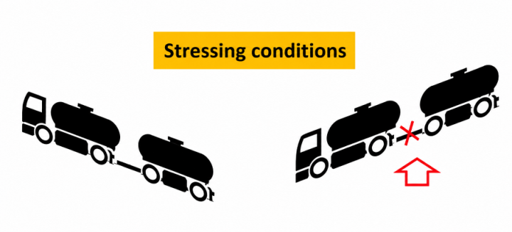
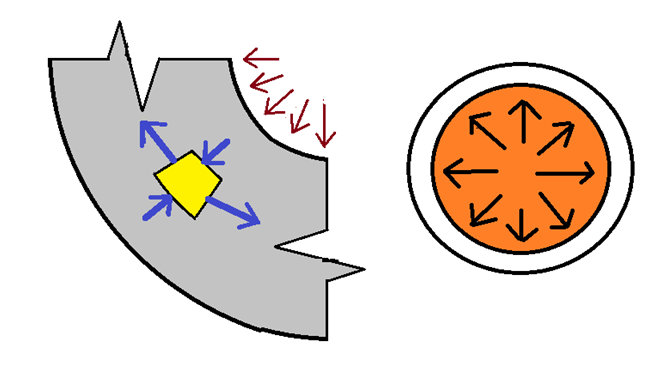
A typical trailer hook suffered a rupture failure during operation, resulting in the uncoupling of part of the vehicle train and a major accident, as shown schematically in Figure 1:

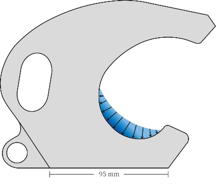
Several analyses were conducted regarding the magnitude of the loads during both acceleration and braking, with the latter proving to be the most critical condition. A schematic drawing of the hook is shown in Figure 2. The hook's geometry is irregular; the contact region has also been sketched and highlighted in the same figure.
A detailed analysis was conducted of the suitability of the hook's constituent material and its properties. The Metrology Laboratory of the Federal University of Espírito Santo (UFES), the Materials Science Laboratory of the Department of Mechanical Engineering, and the Institute of Technology (ITUFES) carried out this work. Chemical analysis of the material, examination of its microstructure, and hardness testing across various parts of the hook revealed no abnormalities.
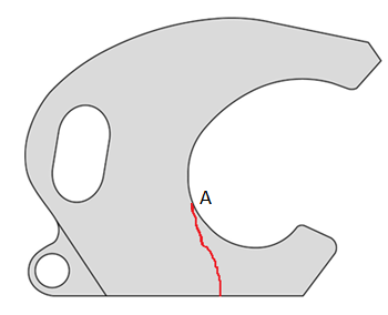
The hypothesis of wear was ruled out due to the existence of an efficient predictive maintenance program maintained by the responsible company, as well as the specific characteristics of the failure; these were inconsistent with frictional wear between the parts – a phenomenon that was also not observed on the mounting pin. Consequently, a structural strength analysis of the design was required to estimate the stresses developed in the hook and to evaluate the adequacy of its dimensions and geometric configuration. Various analyses regarding load magnitudes during both acceleration and braking were conducted; the latter condition proved to be the most critical, explaining the formation of a crack that propagated from point A – located in the contact area between the hook and the pin – toward the mounting edge situated on the lower horizontal line shown in Figure 3.


Numerical modeling was performed using custom software based on the Boundary Element Method for solving linear elastic problems, governed by the Navier’s equation, given by Eq. (9). Quadratic isoparametric elements were employed, and the hook was analyzed under a plane stress state.
To ensure result convergence and stability, meshes with 40, 80, and 120 boundary elements were tested; the results obtained with the finer mesh were deemed sufficiently accurate. Internal stress results were derived via computational post-processing – mapping the internal stress distribution using 100 points, concentrated primarily in the region near the failure site.
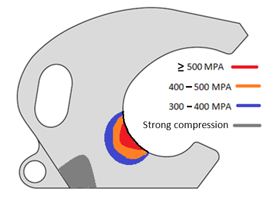
The maximum distortion energy criterion or Von Mises criterion 19 was used to evaluate combined stresses. The results revealed high equivalent stress values, the schematic distribution of which is shown in Figure 4.

The tensile and yield strengths were estimated in the laboratory at 897 MPa and 673 MPa, respectively. Values on the order of 520 MPa were identified at several points in the region near collapse. As the problem is highly dynamic, checking for fatigue under repeated loading indicated an inadequate safety factor against fatigue in the design.
It is worth noting that, as expected, predominant compressive stresses occurred along the horizontal edge at the hook's mounting base. However, high tensile normal stresses were observed along the curved surface in the failure region. To some extent, the contact area between the hook and the pin behaves roughly like a cylinder subjected to compression, where high circumferential tensile stresses arise 20. The emergence of tensile stresses promotes fatigue crack growth, reinforcing the conclusion that this phenomenon caused the failure.

To conclude this example, the BEM model's operational simplicity is highlighted. Processing the input data describing the body's geometry was very straightforward, as was obtaining stress and displacement values. Values at arbitrary internal points within the region of interest were likewise obtained efficiently.
This second example consists of a duct from the thermal system of a nuclear installation and was analyzed using the Finite Element Method to examine the non-stationary cooling process. Because nuclear components require a high level of safety and no analytical solutions are available, the engineering staff opted to compare the axisymmetric FEM model with a similar BEM model. The sudden influx of coolant flow into its interior was the scenario selected for analysis. In this case, the problem is described by the well-known transient heat diffusion equation, presented in Eq. (1) 21, 22.
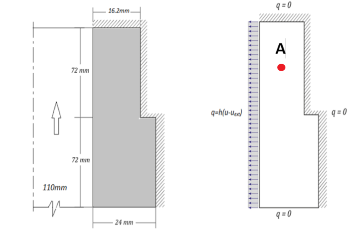
The pipe walls have varying thicknesses, and the length of the section under analysis is 144 mm, as shown on the left-hand side of Figure 6. Other geometric characteristics of the chosen section of revolution are also shown in same figure. The problem can be treated as axisymmetric, since the loads and geometry permit a simplified formulation compared with a three-dimensional model.

The duct is initially at a temperature of 293°C. The liquid flows continuously at 21°C. The outer walls of the duct are insulated, with the Neumann boundary condition equal to zero. However, on the inner walls, where the tube subtly receives the flow of cooling liquid, producing thermal shock, the boundary conditions are convective (Robin condition). Thus, data such as the film coefficient, thermal conductivity, fluid density, and specific heat were made available. The upper and lower horizontal edges are subject to the same condition, characterizing a long pipe of which only a limited section was selected for analysis. All these conditions are shown on the right-hand-side of Figure 6.
The FEM computational modeling employed 2,160 four-node, axisymmetric, quadratic, self-adaptive solid elements. The time-stepping increment used was 0.05 s. In contrast, the discrete BEM model utilized 70 linear isoparametric boundary elements with a time step of 4.0 seconds. To develop the transient BEM model – specifically to construct a thermal inertia matrix – the Dual Reciprocity technique was employed, which required 18 internal interpolating points to ensure faithful representation of internal constitutive properties and adequate response stabilization upon refinement. Dual Reciprocity utilizes a steady-state fundamental solution 23 and, at the time this problem was solved, emerged as an attractive option for an effective, simpler numerical solution in time-dependent cases. Currently, an alternative model known as the Direct Integration Method 24, 25 constructs thermal inertia matrices with greater robustness and superior numerical precision.
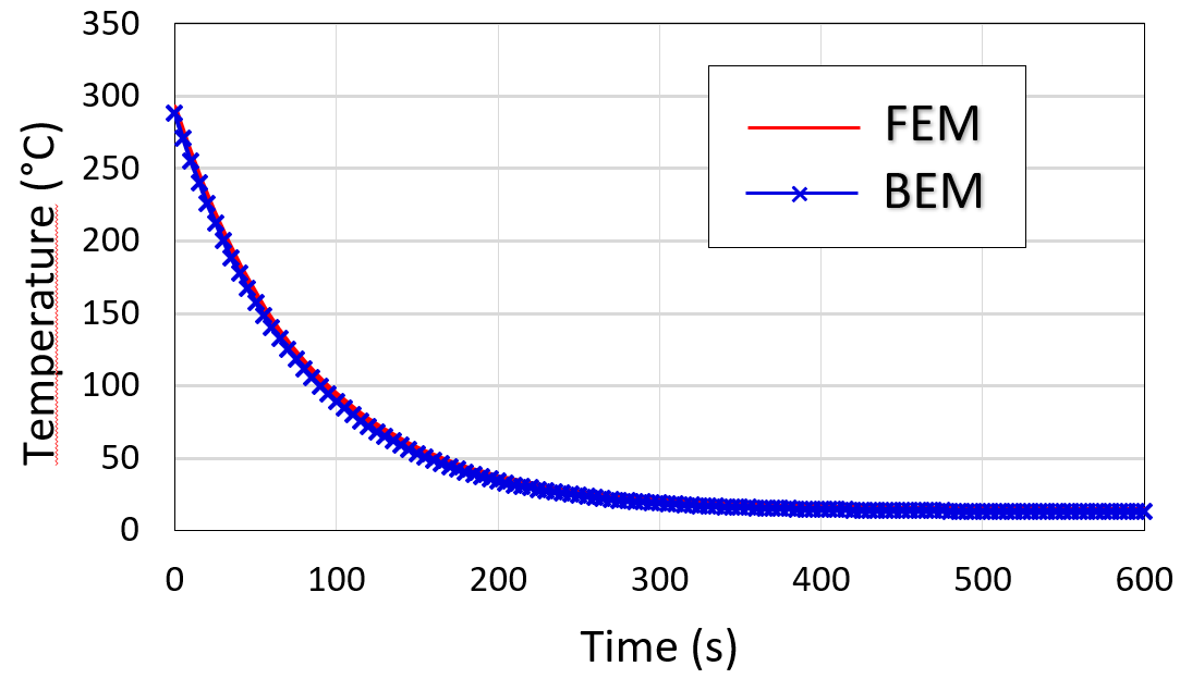
Numerical results were achieved for many points, but to illustrate this analysis, just the evolution of temperature over time at point A is presented in Figure 7. Good agreement between the BEM and FEM results is observed, highlighting that the BEM model was much simpler and thus required much less computational time.

Thus, given the agreement between the results, the simulation using the BEM achieved its objectives, thereby validating the accuracy of the axisymmetric modeling performed with the FEM for other subsystems of the same plant. Due to the high safety requirements for nuclear components and the lack of available analytical solutions, those responsible opted to compare an axisymmetric FEM model with a BEM model – the latter being known for its simplicity and robustness. This alternative was chosen over an evaluation using a three-dimensional finite element model, a common procedure in design engineering when analyzing axisymmetric problems.
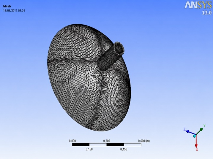
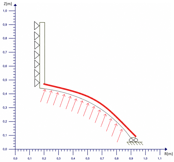
Now a stress analysis is performed in a nozzle-pressure vessel connection. This case was initially solved using ANSYS FEM software with three-dimensional solid finite elements due to a series of operational problems encountered with the axisymmetric code. There were also a series of uncertainties in its results, which motivated the comparison with BEM. As in the first example, this is a static analysis of an elastic problem governed by the Navier equation (see Eq. (9)). Figure 8 shows the geometric features of this case.
The problem at hand prompted a master's thesis project in which the company's design engineer decided to use the axisymmetric elastic BEM model to compare results with those previously obtained using FEM.
The behavior of displacements and stresses was examined in the nozzle-to-head connection region of a pressure vessel subjected to an internal pressure load of 1 Pa, as shown schematically in Figure 9. The region inward of the nozzle's axis of revolution was treated as fixed, and displacements in the head section were constrained in the Y and Z directions.
The pressure vessel's nozzle-to-head connection was characterized by the following dimensions: wall thickness = 20.00 mm; inner radius = 488.50 mm; outer radius = 505.00 mm; and a distance of 34.00 mm between the nozzle's inner surface and the axis of rotation. The boundary element mesh used for the simulation consists of 100 equal-sized isoparametric quadratic elements, with double nodes at the corners.

The behavior of stresses is examined in the nozzle-head connection region of a pressure vessel subjected to an internal pressure load, schematically represented in the figure. The BEM model is very simple. The region inside the axis of revolution of the nozzle was considered fixed and the positions in the head part were constrained in the Y and Z directions.

Figure 10 shows the results for the von Mises equivalent stresses at nodal points on the outer surface of the curved boundary for both methods (line highlighted in red). The larger values occur at the edge of the head and not near the nozzle. The agreement of the results was surprising, although relevant differences were observed at some points near the nozzle.
The displacement values were also quite close, confirming the similarity of the results obtained with the BEM and FEM – despite the use of different models – as they are equivalent given the axisymmetric nature of the problem at hand.
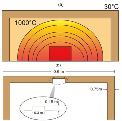
This example addresses another important aspect of thermal transients: some constitutive materials lose their thermal properties due to large variations in heat fluxes, and this phenomenon needs to be checked 26. Usually, these problems are reported when a cooling or ventilation system fails, but similar situations can occur. Here, the problem concerns a protective wall for a blast furnace chamber made of refractory bricks.
These bricks occasionally come loose for various reasons and are subject to several analyses, including thermal fatigue. The value of the thermal transient produced by the reduction in the thickness of the refractory, which reaches high values, is of interest here. Thermal simulation of the transient enables defining the actions to be taken to address the failure, thereby avoiding overheating of components and the environment.
The chamber is schematized, as shown in Figure 11. The internal temperature is 1000 °C, and the external temperature is 30 °C. Although the problem is three-dimensional, a suitable simplification can be assumed by considering it in two dimensions. Symmetry conditions can be applied to the problem, simplifying its numerical model. The steady-state temperature profile is calculated at the boundary and internally, with the latter serving as initial conditions for solving the new problem.
For the numerical simulation of this problem, three finer BEM meshes were tested to evaluate the convergence of the results. The finer mesh has 172 linear boundary elements and 254 internal interpolation points. At these points, the initial conditions are defined, corresponding to the temperature values obtained from the solution of the regular problem without the cut.
Unfortunately, it was not possible to compare results using different methods. The FEM model employed previously does not return satisfactory results. It is well known that the accuracy of FEM in determining internal heat fluxes is inferior to that of BEM; however, the engineers' inexperience in using FEM codes for simulating thermal problems is also a relevant factor in explaining the failure of previous simulations.
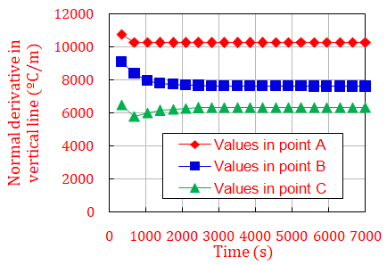
To illustrate the BEM results, three points of the new boundary in which the highest values of the normal derivative occur are highlighted in Figure 12. The response values for these points are presented in Figure 13.


The points closer to the corner yield even higher values but were not considered due to potential inaccuracies arising from the double nodes. The same one presented above is noteworthy regarding an initial peak in the flux value before the new equilibrium values were established. At point B, the transient peak was about 30% higher than the steady-state value, and at point A, it was about 13% higher. This highlights the importance of monitoring thermal transients in heat fluxes, since solid surfaces can suffer significant thermal losses due to changes in their mechanical properties induced by high heat fluxes.
This article presented four applications of the Boundary Element Method (BEM) to engineering problems. These are significant cases demonstrating its versatility and attractive computational simplicity compared to other methods. Mesh generation involves a simple, rapid process with a very low likelihood of error.
Given that the problem dimensions were modest and the analyses were limited to two-dimensional cases, processing time was minimal; consequently, the matrices not being sparse had no significant impact. Despite the challenging applications in modern engineering that demand substantial computational effort, many important problems that are not large-scale are accessible to discrete methods, such as the boundary element method, because the computational capabilities of machines are very large.
Otherwise, as previously noted, some of these problems were addressed to meet stringent design safety requirements-specifically, to verify results obtained through other methods and to account for inaccuracies and uncertainties that can affect the design of critical equipment and complex processes, particularly when only a single numerical technique is used.
On the other hand, it is worth noting that no single method is superior in terms of both accuracy and computational cost across all applications. Nevertheless, the qualities of the BEM are often underestimated or unknown to engineers in general, despite numerous examples of its excellent performance across various engineering fields.
| [1] | Levy, H., Lessman, F., Finite Difference Equations, Dover Publ., New York, 1992. | ||
| In article | |||
| [2] | Reddy, J. N., An Introduction to the Finite Element Method, McGraw Hill, 1993. | ||
| In article | |||
| [3] | Moukalled, F., Mangani, L., Darwish, M., The Finite Volume Method in Computational Fluid Dynamics, Springer, 2015. | ||
| In article | View Article | ||
| [4] | Brebbia, C. A., Telles, J. C. F., Wrobel, L. C., Boundary Element Techniques, Springer Verlag, Berlin Heidelberg, 1984. | ||
| In article | View Article | ||
| [5] | Kythe, P., An Introduction to Boundary Element Methods, Taylor & Francis, 1995. | ||
| In article | View Article PubMed | ||
| [6] | Brebbia, C. A., Walker, S., The Boundary Element Techniques in Engineering, Newnes Butterworths, 1980. | ||
| In article | |||
| [7] | Loeffler, C. F., "A Recursive Application of the Integral Equation in the Boundary Element Method", Engineering Analysis with Boundary Elements. | ||
| In article | |||
| [8] | Ramos, V. E. S., Loeffler, C. F., Mansur, W. J., "Recursive Procedure of Boundary Element Method Applied to Poisson’s Problems", Engineering Analysis with Boundary Elements. | ||
| In article | |||
| [9] | Barcelos, H. M., Loeffler, C. F., Lara, L. O. C., Mansur, W. J., "Recursive Boundary Element Procedure for Computation of Internal Directional Derivatives in Homogeneous Laplace’s Problems Solved by the Finite Element Method", Engineering Analysis with Boundary Elements. | ||
| In article | |||
| [10] | Loeffler, C. F., Lara, L. O. C., Moura, L. C., Stikan, R. P., "Solving Slender Axisymmetric Structures Using the Boundary Element Method", Engineering Analysis with Boundary Elements. | ||
| In article | |||
| [11] | Almeida, L. A., Campos, L. S., Loeffler, C. F., Albuquerque, E. L., "A Fast Boundary Element Method Using Direct Interpolation and Hierarchical Matrices for Efficient Matrix Assembly and Computation", Computers & Mathematics with Applications. | ||
| In article | |||
| [12] | Liu, Y., Fast Multipole Boundary Element Method: Theory and Applications in Engineering, Cambridge University Press, 2009. | ||
| In article | View Article | ||
| [13] | Schiara, L. S., Paschoalini, A. T., "A Detailed Implementation of Multithreading and Out-of-Core Computation to the Conventional Boundary Element Algorithm with Minimum Code Changes", Journal of the Brazilian Society of Mechanical Sciences and Engineering. | ||
| In article | |||
| [14] | Campos, L. S., Loeffler, C. F., "A New Strategy for a Faster Assembly of the Boundary Element Matrices", Computers and Mathematics with Applications. | ||
| In article | |||
| [15] | Rubinstein, M. F., Matrix Computer Analysis of Structures, Prentice Hall, London, 1966. | ||
| In article | |||
| [16] | Holman, J. P., Heat Transfer, McGraw Hill-Kukagusha, Tokyo, 1981. | ||
| In article | |||
| [17] | Buhmann, M. D., Radial Basis Functions: Theory and Implementations, Cambridge University Press, 2003. | ||
| In article | View Article PubMed | ||
| [18] | Loeffler, C. F., Zamprogno, L., Bulcão, A., Mansur, W. J., "Performance of Compact Radial Basis Functions Associated with the Direct Interpolation Boundary Element Method in Potential Problems", CMES, 113(3), 387-412. | ||
| In article | |||
| [19] | Juvinall, R. C., Engineering Considerations of Stress, Strain and Strength, McGraw Hill, New York, 1967. | ||
| In article | |||
| [20] | Den Hartog, J. P., Advanced Strength of Materials, Over Publ., 1984. | ||
| In article | |||
| [21] | Bejan, A., Heat Transfer, John Wiley and Sons, 1993. | ||
| In article | |||
| [22] | Holman, J. P., Heat Transfer, McGraw Hill-Kukagusha, Tokyo, 1981. | ||
| In article | |||
| [23] | Ramachandran, P. A., Boundary Element Methods in Transport Phenomena, Elsevier Applied Science, 1994. | ||
| In article | |||
| [24] | Loeffler, C. F., Mansur, W. J., "A Regularization Scheme Applied to the Direct Interpolation Boundary Element Technique with Radial Basis Functions for Solving Eigenvalue Problem", Engineering Analysis with Boundary Elements, 74, 14–18, 2017. | ||
| In article | View Article | ||
| [25] | Loeffler, C. F., Cruz, A. L., Bulcão, A., "Direct Use of Radial Basis Interpolation Functions for Modelling Source Terms with the Boundary Element Method", Engineering Analysis with Boundary Elements, 50, 97–108, 2015. | ||
| In article | View Article | ||
| [26] | Akishev, A. K., Fomenko, S. M., Tolendiuly, S., "Effect of Refractory Thermal Stresses and Parameters on Development of the Internal Temperature Field", Refractories and Industrial Ceramics. | ||
| In article | |||
Published with license by Science and Education Publishing, Copyright © 2026 Carlos Friedrich Loeffler and Thiago Galdino Balista
 This work is licensed under a Creative Commons Attribution 4.0 International License. To view a copy of this license, visit
http://creativecommons.org/licenses/by/4.0/
This work is licensed under a Creative Commons Attribution 4.0 International License. To view a copy of this license, visit
http://creativecommons.org/licenses/by/4.0/
| [1] | Levy, H., Lessman, F., Finite Difference Equations, Dover Publ., New York, 1992. | ||
| In article | |||
| [2] | Reddy, J. N., An Introduction to the Finite Element Method, McGraw Hill, 1993. | ||
| In article | |||
| [3] | Moukalled, F., Mangani, L., Darwish, M., The Finite Volume Method in Computational Fluid Dynamics, Springer, 2015. | ||
| In article | View Article | ||
| [4] | Brebbia, C. A., Telles, J. C. F., Wrobel, L. C., Boundary Element Techniques, Springer Verlag, Berlin Heidelberg, 1984. | ||
| In article | View Article | ||
| [5] | Kythe, P., An Introduction to Boundary Element Methods, Taylor & Francis, 1995. | ||
| In article | View Article PubMed | ||
| [6] | Brebbia, C. A., Walker, S., The Boundary Element Techniques in Engineering, Newnes Butterworths, 1980. | ||
| In article | |||
| [7] | Loeffler, C. F., "A Recursive Application of the Integral Equation in the Boundary Element Method", Engineering Analysis with Boundary Elements. | ||
| In article | |||
| [8] | Ramos, V. E. S., Loeffler, C. F., Mansur, W. J., "Recursive Procedure of Boundary Element Method Applied to Poisson’s Problems", Engineering Analysis with Boundary Elements. | ||
| In article | |||
| [9] | Barcelos, H. M., Loeffler, C. F., Lara, L. O. C., Mansur, W. J., "Recursive Boundary Element Procedure for Computation of Internal Directional Derivatives in Homogeneous Laplace’s Problems Solved by the Finite Element Method", Engineering Analysis with Boundary Elements. | ||
| In article | |||
| [10] | Loeffler, C. F., Lara, L. O. C., Moura, L. C., Stikan, R. P., "Solving Slender Axisymmetric Structures Using the Boundary Element Method", Engineering Analysis with Boundary Elements. | ||
| In article | |||
| [11] | Almeida, L. A., Campos, L. S., Loeffler, C. F., Albuquerque, E. L., "A Fast Boundary Element Method Using Direct Interpolation and Hierarchical Matrices for Efficient Matrix Assembly and Computation", Computers & Mathematics with Applications. | ||
| In article | |||
| [12] | Liu, Y., Fast Multipole Boundary Element Method: Theory and Applications in Engineering, Cambridge University Press, 2009. | ||
| In article | View Article | ||
| [13] | Schiara, L. S., Paschoalini, A. T., "A Detailed Implementation of Multithreading and Out-of-Core Computation to the Conventional Boundary Element Algorithm with Minimum Code Changes", Journal of the Brazilian Society of Mechanical Sciences and Engineering. | ||
| In article | |||
| [14] | Campos, L. S., Loeffler, C. F., "A New Strategy for a Faster Assembly of the Boundary Element Matrices", Computers and Mathematics with Applications. | ||
| In article | |||
| [15] | Rubinstein, M. F., Matrix Computer Analysis of Structures, Prentice Hall, London, 1966. | ||
| In article | |||
| [16] | Holman, J. P., Heat Transfer, McGraw Hill-Kukagusha, Tokyo, 1981. | ||
| In article | |||
| [17] | Buhmann, M. D., Radial Basis Functions: Theory and Implementations, Cambridge University Press, 2003. | ||
| In article | View Article PubMed | ||
| [18] | Loeffler, C. F., Zamprogno, L., Bulcão, A., Mansur, W. J., "Performance of Compact Radial Basis Functions Associated with the Direct Interpolation Boundary Element Method in Potential Problems", CMES, 113(3), 387-412. | ||
| In article | |||
| [19] | Juvinall, R. C., Engineering Considerations of Stress, Strain and Strength, McGraw Hill, New York, 1967. | ||
| In article | |||
| [20] | Den Hartog, J. P., Advanced Strength of Materials, Over Publ., 1984. | ||
| In article | |||
| [21] | Bejan, A., Heat Transfer, John Wiley and Sons, 1993. | ||
| In article | |||
| [22] | Holman, J. P., Heat Transfer, McGraw Hill-Kukagusha, Tokyo, 1981. | ||
| In article | |||
| [23] | Ramachandran, P. A., Boundary Element Methods in Transport Phenomena, Elsevier Applied Science, 1994. | ||
| In article | |||
| [24] | Loeffler, C. F., Mansur, W. J., "A Regularization Scheme Applied to the Direct Interpolation Boundary Element Technique with Radial Basis Functions for Solving Eigenvalue Problem", Engineering Analysis with Boundary Elements, 74, 14–18, 2017. | ||
| In article | View Article | ||
| [25] | Loeffler, C. F., Cruz, A. L., Bulcão, A., "Direct Use of Radial Basis Interpolation Functions for Modelling Source Terms with the Boundary Element Method", Engineering Analysis with Boundary Elements, 50, 97–108, 2015. | ||
| In article | View Article | ||
| [26] | Akishev, A. K., Fomenko, S. M., Tolendiuly, S., "Effect of Refractory Thermal Stresses and Parameters on Development of the Internal Temperature Field", Refractories and Industrial Ceramics. | ||
| In article | |||