Accurately determining the bearing capacity of shallow foundations is essential in geotechnical engineering. This article proposes an approach using artificial neural networks (ANNs) to estimate the bearing capacity of a continuous footing based on the geotechnical characteristics of the Daraal Peulh site (Senegal). A database of 250 samples was compiled by varying cohesion, the angle of internal friction, the footing width, and the embedment depth. The target values were generated by an equiprobable random mixture of the Terzaghi and Meyerhof formulas. A multilayer perceptron with a hidden layer of 12 neurons, trained using the Levenberg-Marquardt algorithm, yielded a mean squared error (MSE) of 45.97 on the training set and 68.73 on the test set, with correlation coefficients of 0.9932 and 0.9871, respectively. Validation on eight independent samples (four from Terzaghi, four from Meyerhof) yielded relative errors ranging from 3.5% to 38%, with a median error of approximately 13%. This study demonstrates that, despite the inherent variability resulting from the combination of the two theories, the RNA is a rapid and sufficiently reliable estimation tool for the soils of Daraal Peulh, within the limits of the parameter ranges studied.
The reliable design of shallow foundations relies on an accurate estimation of the soil’s bearing capacity. Conventional analytical methods—Terzaghi 1 and Meyerhof 2—remain the standard in practice, but they rely on simplifying assumptions (homogeneous soil, centered vertical load, idealized failure mechanisms) and can lead to significantly different results for the same set of parameters, with no objective criterion for choosing between the two formulations. In situ or laboratory tests, while more direct, remain costly and time-consuming, particularly in contexts where regional geotechnical databases are scarce—as is the case at the DaraalPeulh site (Thiès, Senegal), for which no specific prediction tool exists to date.
Artificial neural networks (ANNs) make it possible to approximate nonlinear relationships between geotechnical parameters and bearing capacity without imposing a functional form a priori 3, 4, and several recent studies attest to their relevance for this type of problem 5, 6, 7, 8. This capability is particularly useful when two competing analytical formulations coexist without consensus on which is best suited to a given site: rather than arbitrarily choosing one of them, this study trains an ANN on targets generated by an equiprobable random mixture of the Terzaghi 1 and Meyerhof 2 formulas, so that the model incorporates the epistemic uncertainty between the two theories rather than favoring one at the expense of the other. It should be noted that this approach is not intended to replace a physical measurement of bearing capacity (such as a plate load test), but rather to produce a rapid estimator—consistent with both theoretical frameworks—over the parameter range specific to the site under study.
The objective of this work is therefore to develop and validate such a model for continuous footings under centered vertical load, as applied to the DaraalPeulh site. Validation is conducted on two levels: internally, through a standard data partition (training, validation, testing); and externally, on eight independent samples from direct shear tests covering both theoretical formulations—a crucial distinction for assessing whether the network truly generalizes beyond its training distribution, rather than simply interpolating within it.
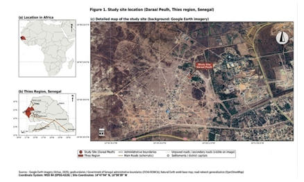
The study site is located in the village of DaraalPeulh, in the Thiès region of Senegal. The study area is defined by the geographic coordinates 14°47'04" N and 16°58'39" W (Figure 1). Soil samples were collected from two distinct areas, a few dozen meters apart, to account for local variability in the materials.

The samples underwent a series of laboratory identification tests: sieve analysis, determination of Atterberg limits, measurement of specific gravity, and direct shear test. The direct shear test was conducted in accordance with current French standards (NF P94-067) 9.
The particle size distribution results and Atterberg limits are presented in the Table1. According to the classification in the Guide to Road Earthworks (GTR), both samples, E1 and E2, are classified in category B6, corresponding to sandy and gravelly soils with plastic clay fines. This classification is justified by a fines content of approximately 27% and a plasticity index slightly greater than 12% for both samples. The methylene blue values (VBS), ranging from 5.30 to 5.72, confirm the presence of a significant active clay fraction. The measured specific weights are 26.5 kN/m³ for E1 and 25.9 kN/m³ for E2, respectively.
It should be noted that the bulk density γ of the soil in situ, which is used in the calculation of bearing capacity, has a measured average value of 22.07 kN/m³.
Direct shear tests were conducted on 30 samples collected from the site. These tests provided the parameters (angle of internal friction φ, cohesion C) that characterize the soil’s strength. A summary of these results is presented in Table 2.
Of these 30 tests, some were used to define the ranges of variation and the linear correlation used to generate the 250 samples in the training set. The remaining tests were reserved to form the independent validation set.
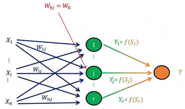
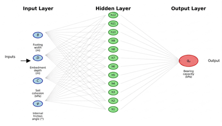
2.2. Artificial Neural Networks (ANNs)An artificial neural network consists of a set of neurons interconnected by synaptic weights, the values of which influence the overall behavior of the structure 10. Building an ANN involves determining its architecture (number of layers, number of neurons per layer) and selecting the activation functions 11. A network typically consists of three types of layers: an input layer, one or more hidden layers, and an output layer, as illustrated in Figure 2.
For a neuron j in the hidden layer, the weighted sum Sj received from the neurons in the previous layer is expressed as (equation(1) ):
 | (1) |
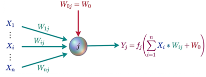
Where n is the number of neurons in the previous layer, X(i) is the output of the i-th neuron, W(ij) is the connection weight between neuron i and neuron j, and W0(,j) is the bias. The output Yj of the neuron is obtained by applying an activation function fj (equation (2)) as illustrated in Figure3:
 | (2) |
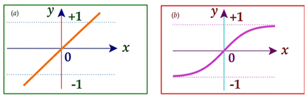
In this work, the activation function chosen for the hidden layer is the symmetric hyperbolic tangent (tansig), defined by:
 | (3) |
Figure 4 (b) illustrates the graph of this activation function.
This function, which is continuous and differentiable, produces an output between –1 and 1, which is suitable for normalizing the input data (which has been previously scaled to the interval [–1,1]). For the output layer, a linear (purelin) activation function is used (Figure 4 a):
 | (4) |
Where b is the result of the weighted sum (including the bias) received by the output neuron, and a is the neuron’s output after applying the activation function. Such a function yields an unbounded output value, which is suitable for predicting a physical quantity such as load-bearing capacity.
The crucial step in developing a neural network is its training, which consists of adjusting the connection weights using an iterative algorithm to minimize the prediction error 12. Let Wij(t) denote the weight connecting neuron j to its input i at time t; the update is performed according to the following equation (5):
 | (5) |
Where is the change in the weight, given by the backpropagation rule from the following equation (6):
 | (6) |
where η is the learning rate and E is the sum of squared errors defined by (equation(7) ):
 | (7) |
where ej is the error at the output of the jth output neuron ( ), Y(j) is the predicted output, and Y(s) is the desired output 13. The backpropagation algorithm, based on the calculation of the error gradient, aims to minimize the error at the network’s output 14, 15.
Among the many optimization algorithms, the Levenberg-Marquardt algorithm was chosen in this study for its fast convergence and robustness in nonlinear regression problems 16. The implementation was carried out in MATLAB using the Neural Network Toolbox (nftool) 17.


Determining the bearing capacity of shallow foundations is a major challenge in geotechnical engineering. It can be evaluated using methods based on laboratory tests, which take into account soil strength parameters such as cohesion C and angle of internal friction φ, or through in situ tests 18. For the purposes of this study, only approaches based on laboratory tests are considered.
Bearing capacity is influenced by several factors, including the foundation’s geometry (shape and dimensions), site conditions, soil mechanical properties, load characteristics, and the possible presence of the water table 19. In this work, the analysis focuses on the main parameters: cohesion C, angle of internal friction φ, footing width B, and embedment depth D.
For a continuous footing subjected to a centered vertical load, the ultimate bearing capacity can be estimated using various analytical methods. In this study, two classical formulations are used: the Terzaghi method 1 and the Meyerhof method 2. The training targets for the neural network are generated by an equiprobable random mixture of the two formulas, in order to make the model robust to uncertainty regarding the most appropriate theoretical method. External validation is performed on eight independent samples, four of which were calculated using Terzaghi’s method and four using Meyerhof’s method.
According to Terzaghi 1, the ultimate failure stress (bearing capacity) is expressed by (equation(8)):
 | (8) |
where:
• c is the soil cohesion [kPa];
• γ is the unit weight of the soil;
• B is the width of the footing [m];
• D is the embedment depth [m];
• Nc, Nq, and Nγ are the bearing capacity factors, which depend solely on the angle of internal friction φ.
These factors are determined based on plasticity theory and limit equilibrium conditions. Terzaghi presented them in the form of charts; they can also be obtained using the following equations:
 | (9) |
 | (10) |
 | (11) |
where KPγ is the passive earth pressure coefficient corresponding to an inclined screen with a soil-screen friction angle δ=φ. According to Coulomb’s theory, this coefficient is given by:
 | (12) |
with the following specific values, in accordance with Terzaghi’s assumptions 1:
 | (13) |
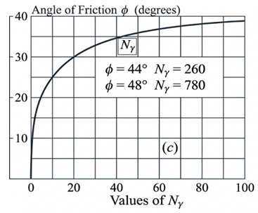
The expression for KPγ with the substitutions α=180°−φ, β=0, and δ=φ leads to an indeterminate form (division by zero) because  . This is why Terzaghi did not use Coulomb’s formula directly to obtain KPγbut instead employed the logarithmic spiral method or the friction circle method, which allows this singularity to be circumvented. In practice, one uses the tabulated values or the abacus from the “Figure5 ), which directly provides the bearing factor Nγas a function of the internal friction angle φ.
In order to remain within the theoretical framework of Terzaghi (1943) and to obtain a simple analytical expression for Nγ, a nonlinear regression was performed using values extracted from the chart at Figure 5. For 0 < φ ≤ 40° ∘, the following relationship was established:
 | (14) |
The coefficient of determination R²= 0.9909 attests to an excellent fit between this expression and the data from the original chart. For φ = 0° (∘), Terzaghi’s theory gives Nγ= 0. This formulation will be used to calculate Nγ in the remainder of the study.

Meyerhof 2 proposes an expression for bearing capacity that incorporates, in addition to the bearing factors, correction coefficients for the foundation shape (sc , sq , s(γ)), the embedment depth (dc, dq, dγ), and the load inclination (ic, iq, iγ ). The ultimate stress is then given by:
 | (15) |
The bearing capacity factors Nc, Nq , and Nγ are given by the following analytical expressions for a continuous footing:
 | (16) |
 (17)
(17)
And the last expression below is itself an approximation:
 | (18) |
where
 | (19) |
• Shape Factors
For a rectangular foundation (W × L), the bearing capacity factors can be obtained by multiplying those of the continuous footing by empirical shape factors:
 (20)
(20)
In the case of a strip footing (B/L→0), the shape factors are ...
• Depth Factors
The influence of the embedment depth can be accounted for by depth factors (for D ≤ B):
 | (21) |
• Inclination factors
For a load inclined at an angle α relative to the vertical, the inclination factors are:
 (22)
(22)

When the load is vertical (in the case of a continuous footing subjected to a centered load with no inclination), α = 0; the inclination factors then become  and do not affect the calculation of the bearing capacity.
• Eccentric Load
For an eccentric load, Meyerhof 2 proposes using an effective width B′ = B − 2e (and similarly for the length), where eis the eccentricity of the load relative to the center of the footing. This effective width is then substituted for B in the expressions for the bearing capacity.
• Case of a continuous footing with a centered vertical load
In this case, B/L → 0 (continuous footing), e = 0 (centered load), and α = 0 (vertical load). The shape and inclination factors are 1, and the bearing capacity reduces to:
 | (23) |
This formulation is used, in addition to Terzaghi’s, for the random generation of training targets (equiprobable mixture) as well as for the calculation of half of the external validation targets (the other half being calculated using Terzaghi).
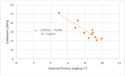
2.4. Database ConstructionThe training dataset is based on a limited number of direct measurements (11 φ–C pairs, Table 3) supplemented by controlled data generation, a common practice when in-situ testing campaigns are costly 7. It is important to specify the dependency structure of this dataset: the internal friction angle φ is randomly generated (normal distribution fitted to the 11 measurements), the cohesion C is derived from it via linear regression (R² = 0.83), while B and D are determined independently of φ and C. The training dataset therefore contains only three true independent degrees of freedom (φ, B, D), since C is a quasi-deterministic function of φ. This dependency—whose consequences for the correlation matrix of the predictions are examined in §3.3.5—constitutes a limitation that should be kept in mind when interpreting the results: the network has never been exposed to independent (φ, C) pairs, unlike what would be observed in real soil, where these two parameters vary in a largely uncorrelated manner 20, 21.
To increase the size of the training set, 250 values of φ were randomly generated. In geotechnical engineering, the variability of strength parameters is frequently modeled using a normal distribution (Gaussian distribution) 22, 23. This assumption is justified by the central limit theorem when the variability results from multiple independent random factors, and it is widely used in reliability analyses and Monte Carlo simulations 8. The parameters of the normal distribution were estimated from the 11 experimental values:
• Mean μφ = 8.245∘
• Standard deviation σφ = 1.35∘
The mathematical equation for generating internal friction angles according to the normal distribution is written as:
 | (24) |
where Z is a reduced-mean normal random variable (mean 0, standard deviation 1), obtained by the inverse transformation of the cumulative distribution function: Z = Φ−1(U), where U is a uniform random variable on [0,1], 1. In practice, we first generate a uniform random variable U (for example, using ALEA() in Excel), then calculate Z using the inverse of the normal distribution function, and finally apply the equation(24 ) . To avoid non-physical values, the random variables were truncated between the minimum of 5.01∘and 9.98∘(common physical limits for an angle of internal friction). The random variables were generated using a spreadsheet (Excel).
The corresponding cohesions were estimated using a linear regression based on the 11 experimental pairs (Figure6 ). The analysis yielded the following equation:
 | (25) |
The coefficient of determination R²= 0.8274 indicates a satisfactory correlation, ensuring the physical consistency of the generated parameter pairs.

The values of B and D were drawn independently from a uniform distribution over their respective intervals [0.20; 1.50] m and [0.20; 1.40] m; draws that did not satisfy the constraint D ≤ B were rejected and removed.
For each combination of the 250 sets of parameters (φ, C, B, D), the target bearing capacity was calculated by randomly selecting (with a probability of 0.5) either Terzaghi’s formula 1 (Equation(8)) or Meyerhof’s formula 2 (Equation(23 ) , adapted for a continuous footing with a centered vertical load). This random mixing approach aims to make the model robust in the face of uncertainty regarding the most appropriate theoretical method. TheTable4 presents an excerpt from the database thus constructed.
To evaluate the model’s generalizability, eight additional samples—not used during training—were collected from the site. Four of these were calculated using Terzaghi’s formula, and the other four using Meyerhof’s formula. Their parameters and target bearing capacities are given in Table 5. These data allow for external validation of the network outside the training set.
Data normalization is an essential preliminary step in training neural networks, particularly when the input variables have different value ranges 24. The use of the tansig activation function (symmetric hyperbolic tangent) in the hidden layer, whose output ranges from –1 to 1, justifies scaling all variables to this interval to avoid saturation effects that could slow down or even halt learning 25.
In this study, the normalization of inputs and targets was performed using MATLAB’s `mapminmax` function. The transformation applied to each variable X is:
 | (26) |
Wherey min = −1 and the parameters xoffset (minimum value of the variable in the training dataset) and gain (scaling factor) are defined by:
 | (27) |
This linear transformation ensures that all normalized values lie within the interval [−1,1].
The minimum and maximum values observed in the database (250 samples) are summarized in Table 4.
The normalization parameters (xoffset and gain) derived from these bounds are presented inError! Reference source not found. This normalization method, automatically implemented by MATLAB’s nftool, preserves the proportional relationships between the values while bringing them to a common scale. It facilitates the convergence of the learning algorithm by ensuring that all parameters contribute in a balanced manner to the initial error 24, 25.
2.6. Network Architecture and Learning ParametersDetermining the optimal neural network architecture is a crucial step in developing a high-performance predictive model 5. The architecture includes the number of hidden layers, the number of neurons per layer, and the choice of activation functions. Several configurations were tested (with the number of neurons in the hidden layer ranging from 5 to 15) to identify the one that minimizes the validation error while avoiding overfitting 5.
The selected architecture consists of:
• An input layer with 4 neurons corresponding to the normalized variables (φnorm, Cnorm, Bnorm, Dnorm);
• A single hidden layer with 12 neurons and a symmetric hyperbolic tangent activation function (tansig);
• An output layer with 1 neuron and a linear activation function (purelin).
The choice of a single hidden layer is justified by the universal approximation theorem of Hornik et al. (1989) 26, according to which a network with a single hidden layer is capable of approximating any continuous function with arbitrary precision, provided there are a sufficient number of neurons in the hidden layer 27. The number of hidden neurons (12) was determined empirically after successive trials on the training dataset, seeking the best compromise between validation error and training stability.
The training parameters were configured as follows 3:
• Optimization algorithm: Levenberg-Marquardt (trainlm), chosen for its fast convergence and robustness in regression problems 28;
• Cost function: Mean squared error (MSE);
• Data split: 70% for training, 15% for validation, and 15% for testing 29;
• Stopping criterion: Earlystopping when the validation error stops decreasing for 6 consecutive epochs, to avoid overfitting 30.
Figure 7 schematically illustrates the architecture of the selected neural network.

The model’s performance was evaluated using two complementary statistical metrics 31:
1. The mean squared error (MSE), which measures the model’s overall accuracy. A value close to zero indicates an excellent fit between the predictions and the target values 32.
 | (28) |
2. The correlation coefficient (R), which measures the strength of the linear relationship between the predicted values and the target values 33:
 | (29) |
An R value close to 1 indicates an excellent correlation between the predictions and the actual values 34.
Model validation was performed at three levels 35:
• Internal validation: The dataset was partitioned into three independent subsets (training, validation, test) to assess the model’s generalization ability 36;
• Regression curve analysis: Visualization of the correlation between predicted values and target values for each subset 37;
• Performance curve analysis: Tracking the evolution of the error as a function of the number of training epochs 38.
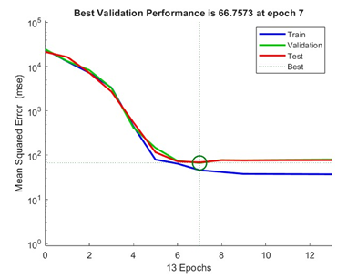
Figure 8 shows the evolution of the neural network’s performance, characterized by the mean squared error (MSE) plotted on a logarithmic scale over a period of 13 epochs. The graph allows us to simultaneously track and compare the convergence dynamics of the training (blue curve), validation (green curve), and test (red curve). The intersection of the black dotted lines, centered on a green circular marker, precisely identifies the optimal inflection point where the best validation performance is achieved—an MSE of 66.7573 at the 7th epoch.

To complement this graphical analysis, all final quantitative metrics as well as the structural distribution of the data are summarized in Table 6.
The final MSEs are 45.97 kPa² on the training set, 66.76 kPa² on the validation set (best), and 68.73 kPa² on the test set, corresponding to RMSEs of 6.8, 8.2, and 8.3 kPa—average relative errors in the range of 2.3 to 2.8% relative to the mean value of qu (≈293 kPa). The difference between the training error and the test error remains moderate, indicating that the model generalizes well despite the variability introduced by mixing the two theoretical formulations. The correlation coefficients (R) are high: 0.9932 for training, 0.9883 for validation, and 0.9871 for testing, confirming the network’s strong predictive ability.
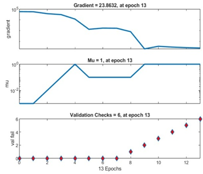
The optimization process and the model’s stopping criteria were rigorously monitored throughout the training epochs. Quantitative details of this temporal evolution are recorded inTable7 , while the graphical dynamics of the key parameters are illustrated by the Figure 9.
Analysis of the Table 7 and the Figure 9 shows that training stopped prematurely at epoch 13 (out of a maximum of 1,000). This convergence is marked by a drastic drop in performance (Mean Squared Error, MSE), which falls from 2.43×10⁴ to 37. At the same time, the control parameter  of the Levenberg-Marquardt algorithm stabilized at 1, while the gradient decreased from 5.92×10⁴ to 23.86. Although the gradient did not reach its target value (10⁻⁷), this behavior is normal: early termination halted the process as soon as the validation error stabilized, before the gradient fully converged, which does not constitute a failure to converge.
In fact, the termination was triggered by the validation checks criterion. As illustrated in
Figure 9, the validation error increased continuously over 6 consecutive epochs (from the 8th to the 13th epoch), reaching the critical failure threshold (val fail = 6). This standard early-stopping mechanism in MATLAB helps prevent overfitting and ensures excellent generalization ability for the model.

 `, and the failure counter for validation checks
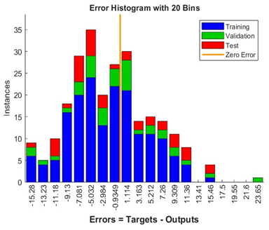
Figure 10 illustrates the error histogram (target – output) for the training, validation, and test sets. The error distribution is generally centered around zero, with a predominance of negative values, indicating a moderate tendency for the model to overestimate the load-bearing capacity.
The majority of errors fall within the interval [-10; 5], with a notable concentration in the classes between -9 and -5, where the number of data points is highest. The frequency of errors gradually decreases toward the extreme values, reflecting the low occurrence of significant deviations between the predicted and target values.
Furthermore, the distribution of errors across the training, validation, and test sets appears uniform, with no notable divergence. The test samples exhibit a distribution comparable to that of the other subsets, with errors predominantly close to zero, confirming the model’s strong generalization ability.
This relatively low dispersion of errors, combined with low mean squared error (MSE) values and high correlation coefficients (R > 0.98), attests to the robustness and reliability of the developed model. The tendency toward overestimation remains moderate and does not significantly impair the overall accuracy of the predictions.


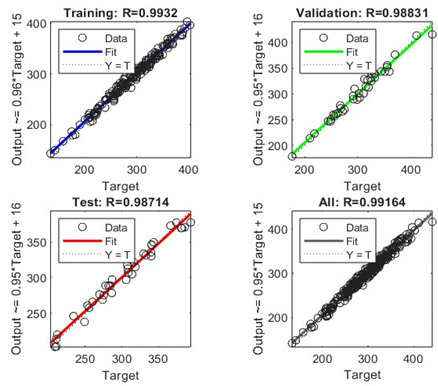
Figure 11 shows, for each set (training, validation, test, and overall), the correlation between the targets and the network’s outputs. The correlation coefficients R are very high: 0.9932 for training, 0.9883 for validation, 0.9871 for testing, and approximately 0.9930 for the overall set. These values, close to 1, indicate an excellent linear correlation between the network’s predictions and the targets derived from the random mixture of the Terzaghi and Meyerhof formulas. The slight dispersion observed on the test set corresponds to the slightly higher MSE on this subset (68.73 versus 45.97 for training). The set of regressions confirms the mixed model’s good predictive ability.
3.2. Derivation of the Overall Equation for the Neural NetworkThe objective of this section is to mathematically express the internal functioning of the developed model, that is to derive the equations linking the network’s inputs to its output, based on the learned parameters (weights and biases). The selected model has the following structure:
• Four inputs corresponding to the parameters: internal friction angle φ (degrees), cohesion C (kPa), embedment depth D (m), and footing width B (m);
• A hidden layer consisting of 12 neurons, with a symmetric hyperbolic tangent activation function (tansig);
• An output layer with a single neuron and a linear activation function (purelin), whose output is the bearing capacity qu.
The calculations are performed in three steps: normalization of the inputs, calculation of the hidden outputs, and then the final denormalized output.
Each raw input  is transformed into the interval [−1,1] using the following formula:
 (30)
(30)
The normalization constants are given in Table 8 Error! Reference source not found.
For each neuron i (i=1,…,12), we calculate the linear combination:
For each neuron i (i=1,…,12), we calculate the linear combination:
 | (31) |
then the neuron’s output:
 | (32) |
The weights  and the biases
  are compiled in the Table 8.
The normalized output (in [−1,1]) is:
 (33)
(33)
with  and the weights
  given in Table 8.
The actual (denormalized) output is obtained by:
 | (34) |
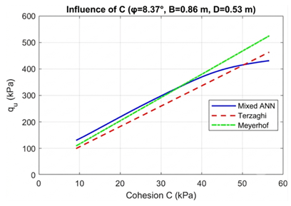
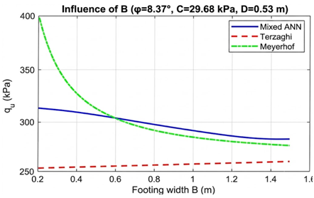
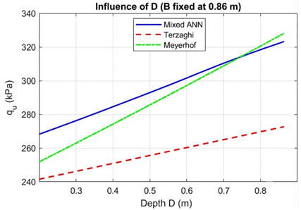
To validate the behavior of the mixed RNA model (trained on the Terzaghi and Meyerhof formulas), a parametric analysis was conducted by varying one parameter at a time, while keeping the others at their average values: φ = 8.37°, C = 29.68 kPa, D = 0.53 m, B = 0.86 m . The results are compared with the predictions of the two theoretical methods.
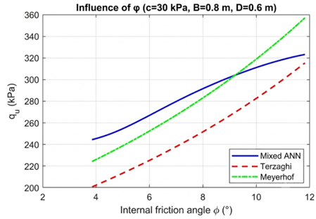
The Figure12 illustrates the variation of the ultimate bearing capacity (qu) as a function of the internal friction angle (φ), for a cohesion fixed at 30 kPa. It shows a monotonic increase in qu with φ for all three models. The mixed RNA model is distinguished by its nonlinear behavior: for φ< 9°, it overestimates the classical models (at 8°: 285 kPa, or +5.3% vs. Meyerhof and +16.3% vs. Terzaghi). Around 9°, Meyerhof’s model exceeds it, and at 12°, it yields the highest value (≈360 kPa), followed by the RNA (≈323 kPa) and Terzaghi (≈315 kPa). The RNA therefore does not act as a simple arithmetic mean, but rather as a smoothed transition envelope between the two theories.

Figure13 illustrates the models’ response to variations in cohesion C. For Terzaghi and Meyerhof, the relationship is strictly linear, whereas the mixed RNA follows a curvilinear profile, with a flattening of the slope at high cohesion values. For C < 45 kPa, the RNA closely follows the Meyerhof curve, slightly overestimating it (at C = 30 kPa: 330 kPa, compared to 325 and 290 kPa for Meyerhof and Terzaghi). Beyond C = 45 kPa, this nonlinearity dampens the growth: at C = 55 kPa, the RNA prediction (≈425 kPa) falls below that of Meyerhof (≈510 kPa) and converges toward Terzaghi (≈450 kPa). The figure thus highlights the flexibility of the multilayer perceptron, which locally shifts from a trend close to Meyerhof’s to one close to Terzaghi’s.

Figure 14 illustrates the impact of the sole width B, revealing a fundamental divergence between the theories: Terzaghi predicts linear growth ( γ term), while Meyerhof implies hyperbolic decay via his corrective shape factors. The mixed RNA closely aligns with Meyerhof’s physics, while smoothing out the extremes. For B = 0.2 m, it mitigates Meyerhof’s singularity (≈400 kPa) by limiting his prediction to 315 kPa. At B ≈ 0.6 m, the RNA and Meyerhof curves intersect at 303 kPa. For B > 0.6 m, both become asymptotic and nearly parallel, with the RNA retaining a slight positive bias (at 1.4 m: 285 kPa versus 278 kPa for Meyerhof). The figure thus demonstrates that the mesh has perfectly incorporated the geometric corrections and Meyerhof’s scale effect, while smoothing out the singularities at the extreme boundaries.

Figure15 illustrates the variation of qu as a function of embedment depth D, confirming a strictly linear increase for all approaches, which validates the stabilizing effect of the lateral surcharge ( ). Subject to the geometric constraint D ≤ B (range from 0.2 to 0.86 m for B = 0.86 m), the mixed RNA slightly overestimates both models over most of the valid domain (0.2 ≤ D ≤ 0.75 m). At D = 0.5 m, the RNA predicts 292 kPa, compared to 286 kPa for Meyerhof and 255 kPa for Terzaghi. For D > 0.75 m, the steeper slope of the Meyerhof model (due to its depth coefficients) causes it to cross the neural network curve at D ≈ 0.77 m (≈315 kPa), beyond which Meyerhof once again outperforms the neural network. The figure thus highlights the network’s ability to follow linear trends while capturing the inflections associated with Meyerhof’s depth corrections.


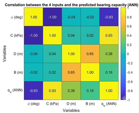
Figure 16 shows the correlation matrix between the input variables and the predicted output (qu, RNA), with coefficients of –0.93 for φ, +0.93 for C, +0.38 for D, and +0.18 for B. A perfect negative correlation (−1.00) is observed between φ and C, resulting from the artificial generation of C from φ during the construction of the database. This redundancy sheds light on the previous results: by varying only φ (§3.3.1) or only C (§3.3.2), the network is forced to evaluate novel pairs, which causes the overestimates and anomalies observed at the boundaries of the graphs. Conversely, the geometric parameters B and D, estimated independently, exhibit much more stable sensitivity profiles (§3.3.3 and §3.3.4). The figure thus allows us to conclude that the model is highly reliable (MSE < 70, R > 0.98) but only for soils whose (φ, C) pairs remain close to the learned statistical relationship, which explains the local deviations observed during external validation on real-world data. For generalization beyond the Daraal Peulh site, a training dataset with independent sampling of φ and C is essential.
3.4. Validation on Independent DataTable 5 (§2.4.2) presents the validation results for eight independent samples. The model achieves an RMSE of 36.6 kPa and a correlation coefficient R ≈ 0.69, which is significantly lower than the R > 0.98 values obtained during the training, validation, and test phases, indicating poorer generalization performance outside the training dataset. The errors vary: they are low for samples 1, 2, 3, and 5 (3.5% to 13.1%), but high for samples 4, 6, 7, and 8 (15% to 38%). This disparity is primarily attributable to the deviation of each (φ,C) pair from the learned relationship  : Sample No. 8 has the largest deviation (24.8 kPa) and the largest error (38.4%), while Sample No. 2 has the smallest deviation (2.1 kPa) and the smallest error (3.5%). However, the match is not perfect (e.g., sample No. 5), suggesting an additional influence of the uneven coverage of the parameter space by the 250 training points. The table also notes that sample No. 1 (φ=11.55°) falls outside the training range (5.01°–9.98°), but its moderate error (9.5%) does not allow for a conclusion regarding the model’s extrapolation capability. In practice, the model proves useful for soils in Daraal Peulh, where the measured torque values remain close to the learned relationship, but its reliability deteriorates significantly outside this range—a limitation to be addressed in a future version of the training dataset.
This study developed an artificial neural network to estimate the bearing capacity of strip footings under a centered vertical load, applied to the Daraal Peulh site (Thiès, Senegal). The model was trained on 250 samples whose target values result from an equiprobable random mixture of the Terzaghi and Meyerhof formulas—an approach aimed at accommodating the uncertainty between the two theories rather than arbitrarily choosing one over the other. It should be noted that this methodological choice makes the model a meta-estimator of the two analytical formulations, rather than a model trained on direct physical measurements of bearing capacity.
The internal performance is satisfactory (R = 0.993 during training, 0.987 during testing), but validation on eight independent samples reveals a notable decline in generalization (R ≈ 0.69, RMSE = 36.6 kPa), with individual errors ranging from 3.5% to 38%. Parametric analysis and the correlation matrix identified the main cause of this degradation: the deterministic quasi- e relationship imposed between φ and C during the generation of the training dataset (r = −1.00) restricts the model’s validity to (φ, C) pairs close to this relationship and produces a systematic overestimation when this constraint is violated—whether in the univariate parametric analysis or for certain external validation samples.
These results suggest that the model’s scope should be qualified: it serves as a rapid and useful estimation tool as a first approximation for soils in Daraal Peulh, where the measured (φ, C) pairs remain close to the learned relationship; however, its generalizability to soils where these two parameters vary independently remains to be demonstrated. Future work should focus primarily on reconstructing a training dataset in which φ and C are sampled independently, on acquiring a larger external validation dataset, and on extending the approach to off-center or inclined load configurations, which were not covered in this study.
| [1] | Terzaghi, K. (1943). Theoretical Soil Mechanics. John Wiley & Sons. | ||
| In article | View Article | ||
| [2] | George Geoffrey Meyerhof. (1963). Some Recent Research on the Bearing Capacity of Foundations. Canadian Geotechnical Journal. 1(1): 16–26. | ||
| In article | View Article | ||
| [3] | Haykin, S. (2009). Neural Networks and Learning Machines (3rd ed.). Pearson Education. | ||
| In article | |||
| [4] | Shahin, M.A., Jaksa, M.B., & Maier, H.R. (2009). Recent advances and future challenges for artificial neural systems in geotechnical engineering applications. Advances in Artificial Neural Systems, 2009, 1-9. | ||
| In article | View Article | ||
| [5] | Goh, A.T.C. (1995). Back-propagation neural networks for modeling complex systems. Artificial Intelligence in Engineering, 9(3), 143–151. | ||
| In article | View Article | ||
| [6] | Moayedi, Hossein & Jahed Armaghani, Danial. (2018). Optimizing an ANN model with ICA for estimating the bearing capacity of driven piles in cohesionless soil. Engineering with Computers, 34. 10.1007/s00366-017-0545-7. | ||
| In article | View Article | ||
| [7] | Moayedi, Hossein, Mosallanezhad, Mansour, A. Rashid, Ahmad Safuan, Wan Jusoh, Wan, and Mu'azu, Mohammed. (2020). A systematic review and meta-analysis of artificial neural network applications in geotechnical engineering: theory and applications. Neural Computing and Applications. 32. 10.1007/s00521-019-04109-9. | ||
| In article | View Article | ||
| [8] | Acharyya, Rana & Dey, Arindam. (2019). Assessment of bearing capacity for strip footings located near a sloping surface using an ANN model. Neural Computing and Applications. 31. 8087–8100. 10.1007/s00521-018-3661-4. | ||
| In article | View Article | ||
| [9] | AFNOR. (1994). NF P94-071-1: Soils: Investigation and Testing—Box Shear Test—Part 1: Direct Shear. French Standardization Association. | ||
| In article | |||
| [10] | McCulloch, W.S., & Pitts, W. (1943). A logical calculus of the ideas immanent in nervous activity. The Bulletin of Mathematical Biophysics, 5(4), 115–133. | ||
| In article | View Article PubMed | ||
| [11] | Rosenblatt, F. (1958). The perceptron: A probabilistic model for information storage and organization in the brain. Psychological Review, 65(6), 386–408. | ||
| In article | View Article PubMed | ||
| [12] | Rumelhart, D.E., Hinton, G.E., & Williams, R.J. (1986). Learning representations by back-propagating errors. *Nature*, 323(6088), 533–536. | ||
| In article | View Article | ||
| [13] | Hagan, M.T., & Menhaj, M.B. (1994). Training feedforward networks with the Marquardt algorithm. IEEE Transactions on Neural Networks, 5(6), 989–993. | ||
| In article | View Article PubMed | ||
| [14] | LeCun, Y., Bengio, Y., & Hinton, G. (2015). Deep learning. Nature, 521(7553), 436–444. | ||
| In article | View Article PubMed | ||
| [15] | Goodfellow, I., Bengio, Y., & Courville, A. (2016). Deep Learning. MIT Press. | ||
| In article | |||
| [16] | Bui, X.N., Muazu, M.A., & Nguyen, H. (2020). Optimizing the Levenberg–Marquardt backpropagation technique for predicting the safety factor of slopes following two-dimensional OptumG2 analysis. Engineering with Computers, 36(3), 941–952. | ||
| In article | View Article | ||
| [17] | MathWorks. (2023). MATLAB Neural Network Toolbox User’s Guide. The MathWorks Inc. | ||
| In article | |||
| [18] | Chwała, M., & Puła, W. (2020). Evaluation of shallow foundation bearing capacity in the case of a two-layered soil and spatial variability in soil strength parameters. PLoS ONE 15(4): e0231992. | ||
| In article | View Article PubMed | ||
| [19] | Pantelidis, L., Meddah, A. The Effect of Loading Inclination and Eccentricity on the Bearing Capacity of Shallow Foundations: A Review. Arch Computat Methods Eng 31, 4189–4208 (2024). | ||
| In article | View Article | ||
| [20] | Skempton, A.W. (1951). The bearing capacity of clays. Proc. Building Research Congress ICE 0 180–189, 1951. | ||
| In article | |||
| [21] | Terzaghi, K., Peck, R.B., & Mesri, G. (1996). Soil Mechanics in Engineering Practice. Wiley. | ||
| In article | |||
| [22] | Phoon, K.K., & Kulhawy, F.H. (1999). Characterization of geotechnical variability. Canadian Geotechnical Journal, 36(4), 612–624. | ||
| In article | View Article | ||
| [23] | Duncan, J.M. (2000). Factors of safety and reliability in geotechnical engineering. Journal of Geotechnical and Geoenvironmental Engineering, 126(4), 307–316. | ||
| In article | View Article | ||
| [24] | Han, J., Kamber, M., & Pei, J. (2011). Data Mining: Concepts and Techniques (3rd ed.). Morgan Kaufmann. | ||
| In article | |||
| [25] | Patro, S. Gopal & Sahu, Dr. Kishore Kumar. (2015). Normalization: A Preprocessing Stage. IARJSET. 20–22. 10.17148/IARJSET.2015.2305. | ||
| In article | View Article | ||
| [26] | Hornik, K., Stinchcombe, M., & White, H. (1989). Multilayer feedforward networks are universal approximators. Neural Networks, 2(5), 359–366. | ||
| In article | View Article PubMed | ||
| [27] | Cybenko, G. (1989). Approximation by superpositions of a sigmoidal function. Mathematics of Control, Signals and Systems, 2(4), 303–314. | ||
| In article | View Article | ||
| [28] | Hagan, M.T., Demuth, H.B., & Beale, M.H. (1996). Neural Network Design. PWS Publishing. | ||
| In article | |||
| [29] | Ripley, B.D. (1996). Pattern Recognition and Neural Networks. Cambridge University Press. | ||
| In article | View Article PubMed | ||
| [30] | Prechelt, L. (1998). Early Stopping—But When?. In: Orr, G.B., Müller, K.R. (eds.) Neural Networks: Tricks of the Trade. Lecture Notes in Computer Science, vol. 1524. Springer, Berlin, Heidelberg. | ||
| In article | View Article | ||
| [31] | Chai, T., & Draxler, R.R. (2014). Root mean square error (RMSE) or mean absolute error (MAE)? Geoscientific Model Development, 7(3), 1247–1250. | ||
| In article | View Article | ||
| [32] | Willmott, C.J., & Matsuura, K. (2005). Advantages of the mean absolute error (MAE) over the root mean square error (RMSE) in assessing average model performance. Climate Research, 30(1), 79–82. | ||
| In article | View Article | ||
| [33] | Legates, D.R., & McCabe, G.J. (1999). Evaluating the use of “goodness-of-fit” measures in hydrologic and hydroclimatic model validation. Water Resources Research, 35(1), 233–241. | ||
| In article | View Article | ||
| [34] | Nash, J.E., & Sutcliffe, J.V. (1970). River flow forecasting through conceptual models, Part I—A discussion of principles. Journal of Hydrology, 10(3), 282–290. | ||
| In article | View Article | ||
| [35] | Ron Kohavi. 1995. A study of cross-validation and bootstrap for accuracy estimation and model selection. In Proceedings of the 14th International Joint Conference on Artificial Intelligence—Volume 2 (IJCAI'95). Morgan Kaufmann Publishers Inc., San Francisco, CA, USA, 1137–1143. | ||
| In article | |||
| [36] | Stone, M. (1974). Cross-validatory choice and assessment of statistical predictions. Journal of the Royal Statistical Society: Series B, 36(2), 111–133. | ||
| In article | View Article | ||
| [37] | Montgomery, D.C., Peck, E.A., & Vining, G.G. (2012). Introduction to Linear Regression Analysis (5th ed.). John Wiley & Sons. | ||
| In article | |||
| [38] | Bishop, C.M. (2006). Pattern Recognition and Machine Learning. Springer. | ||
| In article | |||
Published with license by Science and Education Publishing, Copyright © 2026 Hamed FALL, Déthié SARR, Lamine BAR and Abdou Aziz WELLE
 This work is licensed under a Creative Commons Attribution 4.0 International License. To view a copy of this license, visit
http://creativecommons.org/licenses/by/4.0/
This work is licensed under a Creative Commons Attribution 4.0 International License. To view a copy of this license, visit
http://creativecommons.org/licenses/by/4.0/
| [1] | Terzaghi, K. (1943). Theoretical Soil Mechanics. John Wiley & Sons. | ||
| In article | View Article | ||
| [2] | George Geoffrey Meyerhof. (1963). Some Recent Research on the Bearing Capacity of Foundations. Canadian Geotechnical Journal. 1(1): 16–26. | ||
| In article | View Article | ||
| [3] | Haykin, S. (2009). Neural Networks and Learning Machines (3rd ed.). Pearson Education. | ||
| In article | |||
| [4] | Shahin, M.A., Jaksa, M.B., & Maier, H.R. (2009). Recent advances and future challenges for artificial neural systems in geotechnical engineering applications. Advances in Artificial Neural Systems, 2009, 1-9. | ||
| In article | View Article | ||
| [5] | Goh, A.T.C. (1995). Back-propagation neural networks for modeling complex systems. Artificial Intelligence in Engineering, 9(3), 143–151. | ||
| In article | View Article | ||
| [6] | Moayedi, Hossein & Jahed Armaghani, Danial. (2018). Optimizing an ANN model with ICA for estimating the bearing capacity of driven piles in cohesionless soil. Engineering with Computers, 34. 10.1007/s00366-017-0545-7. | ||
| In article | View Article | ||
| [7] | Moayedi, Hossein, Mosallanezhad, Mansour, A. Rashid, Ahmad Safuan, Wan Jusoh, Wan, and Mu'azu, Mohammed. (2020). A systematic review and meta-analysis of artificial neural network applications in geotechnical engineering: theory and applications. Neural Computing and Applications. 32. 10.1007/s00521-019-04109-9. | ||
| In article | View Article | ||
| [8] | Acharyya, Rana & Dey, Arindam. (2019). Assessment of bearing capacity for strip footings located near a sloping surface using an ANN model. Neural Computing and Applications. 31. 8087–8100. 10.1007/s00521-018-3661-4. | ||
| In article | View Article | ||
| [9] | AFNOR. (1994). NF P94-071-1: Soils: Investigation and Testing—Box Shear Test—Part 1: Direct Shear. French Standardization Association. | ||
| In article | |||
| [10] | McCulloch, W.S., & Pitts, W. (1943). A logical calculus of the ideas immanent in nervous activity. The Bulletin of Mathematical Biophysics, 5(4), 115–133. | ||
| In article | View Article PubMed | ||
| [11] | Rosenblatt, F. (1958). The perceptron: A probabilistic model for information storage and organization in the brain. Psychological Review, 65(6), 386–408. | ||
| In article | View Article PubMed | ||
| [12] | Rumelhart, D.E., Hinton, G.E., & Williams, R.J. (1986). Learning representations by back-propagating errors. *Nature*, 323(6088), 533–536. | ||
| In article | View Article | ||
| [13] | Hagan, M.T., & Menhaj, M.B. (1994). Training feedforward networks with the Marquardt algorithm. IEEE Transactions on Neural Networks, 5(6), 989–993. | ||
| In article | View Article PubMed | ||
| [14] | LeCun, Y., Bengio, Y., & Hinton, G. (2015). Deep learning. Nature, 521(7553), 436–444. | ||
| In article | View Article PubMed | ||
| [15] | Goodfellow, I., Bengio, Y., & Courville, A. (2016). Deep Learning. MIT Press. | ||
| In article | |||
| [16] | Bui, X.N., Muazu, M.A., & Nguyen, H. (2020). Optimizing the Levenberg–Marquardt backpropagation technique for predicting the safety factor of slopes following two-dimensional OptumG2 analysis. Engineering with Computers, 36(3), 941–952. | ||
| In article | View Article | ||
| [17] | MathWorks. (2023). MATLAB Neural Network Toolbox User’s Guide. The MathWorks Inc. | ||
| In article | |||
| [18] | Chwała, M., & Puła, W. (2020). Evaluation of shallow foundation bearing capacity in the case of a two-layered soil and spatial variability in soil strength parameters. PLoS ONE 15(4): e0231992. | ||
| In article | View Article PubMed | ||
| [19] | Pantelidis, L., Meddah, A. The Effect of Loading Inclination and Eccentricity on the Bearing Capacity of Shallow Foundations: A Review. Arch Computat Methods Eng 31, 4189–4208 (2024). | ||
| In article | View Article | ||
| [20] | Skempton, A.W. (1951). The bearing capacity of clays. Proc. Building Research Congress ICE 0 180–189, 1951. | ||
| In article | |||
| [21] | Terzaghi, K., Peck, R.B., & Mesri, G. (1996). Soil Mechanics in Engineering Practice. Wiley. | ||
| In article | |||
| [22] | Phoon, K.K., & Kulhawy, F.H. (1999). Characterization of geotechnical variability. Canadian Geotechnical Journal, 36(4), 612–624. | ||
| In article | View Article | ||
| [23] | Duncan, J.M. (2000). Factors of safety and reliability in geotechnical engineering. Journal of Geotechnical and Geoenvironmental Engineering, 126(4), 307–316. | ||
| In article | View Article | ||
| [24] | Han, J., Kamber, M., & Pei, J. (2011). Data Mining: Concepts and Techniques (3rd ed.). Morgan Kaufmann. | ||
| In article | |||
| [25] | Patro, S. Gopal & Sahu, Dr. Kishore Kumar. (2015). Normalization: A Preprocessing Stage. IARJSET. 20–22. 10.17148/IARJSET.2015.2305. | ||
| In article | View Article | ||
| [26] | Hornik, K., Stinchcombe, M., & White, H. (1989). Multilayer feedforward networks are universal approximators. Neural Networks, 2(5), 359–366. | ||
| In article | View Article PubMed | ||
| [27] | Cybenko, G. (1989). Approximation by superpositions of a sigmoidal function. Mathematics of Control, Signals and Systems, 2(4), 303–314. | ||
| In article | View Article | ||
| [28] | Hagan, M.T., Demuth, H.B., & Beale, M.H. (1996). Neural Network Design. PWS Publishing. | ||
| In article | |||
| [29] | Ripley, B.D. (1996). Pattern Recognition and Neural Networks. Cambridge University Press. | ||
| In article | View Article PubMed | ||
| [30] | Prechelt, L. (1998). Early Stopping—But When?. In: Orr, G.B., Müller, K.R. (eds.) Neural Networks: Tricks of the Trade. Lecture Notes in Computer Science, vol. 1524. Springer, Berlin, Heidelberg. | ||
| In article | View Article | ||
| [31] | Chai, T., & Draxler, R.R. (2014). Root mean square error (RMSE) or mean absolute error (MAE)? Geoscientific Model Development, 7(3), 1247–1250. | ||
| In article | View Article | ||
| [32] | Willmott, C.J., & Matsuura, K. (2005). Advantages of the mean absolute error (MAE) over the root mean square error (RMSE) in assessing average model performance. Climate Research, 30(1), 79–82. | ||
| In article | View Article | ||
| [33] | Legates, D.R., & McCabe, G.J. (1999). Evaluating the use of “goodness-of-fit” measures in hydrologic and hydroclimatic model validation. Water Resources Research, 35(1), 233–241. | ||
| In article | View Article | ||
| [34] | Nash, J.E., & Sutcliffe, J.V. (1970). River flow forecasting through conceptual models, Part I—A discussion of principles. Journal of Hydrology, 10(3), 282–290. | ||
| In article | View Article | ||
| [35] | Ron Kohavi. 1995. A study of cross-validation and bootstrap for accuracy estimation and model selection. In Proceedings of the 14th International Joint Conference on Artificial Intelligence—Volume 2 (IJCAI'95). Morgan Kaufmann Publishers Inc., San Francisco, CA, USA, 1137–1143. | ||
| In article | |||
| [36] | Stone, M. (1974). Cross-validatory choice and assessment of statistical predictions. Journal of the Royal Statistical Society: Series B, 36(2), 111–133. | ||
| In article | View Article | ||
| [37] | Montgomery, D.C., Peck, E.A., & Vining, G.G. (2012). Introduction to Linear Regression Analysis (5th ed.). John Wiley & Sons. | ||
| In article | |||
| [38] | Bishop, C.M. (2006). Pattern Recognition and Machine Learning. Springer. | ||
| In article | |||