1. Introduction

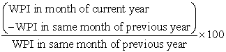
Inflation is the percentage change in the value of the Wholesale Price Index (WPI) on a year-on year basis. It effectively measures the change in the prices of a basket of goods and services in a year. In , inflation is calculated by taking the WPI as base. Thus, the formula for calculating Inflation is:

Inflation occurs due to an imbalance between demand and supply of money, changes in production and distribution cost or increase in taxes on products. When economy experiences inflation, i.e. when the price level of goods and services rises, the value of currency reduces. This means now each unit of currency buys fewer goods and services.

It has its worst impact on consumers. High prices of day-to-day goods make it difficult for consumers to afford even the basic commodities in life. This leaves them with no choice but to ask for higher incomes. Hence the government tries to keep inflation under control.

Contrary to its negative effects, a moderate level of inflation characterizes a good economy. An inflation rate of 2 or 3% is beneficial for an economy as it encourages people to buy more and borrow more, because during times of lower inflation, the level of interest rates also remains low. Hence the government as well as the central bank always strives to achieve a limited level of inflation.

In hardly does the day go by without government officials, politicians and economist talking about inflation. In some cases we are told inflation is high for a particular month and low for another month. There are several important variables that help to describe the state of an economy. These include inflation, unemployment, the budget balance, the interest rates, and the balance of payments. Inflation may be defined as a rise in the average level of a group of prices in a country. The term is sometimes restricted to prolonged or sustained rises. Inflation creates a problem because the purchasing power of money falls as the price level rises. It imposes an opportunity cost on holders of money. Thus inflation ^[1] will reduce the real value of money wage, and savings accounts making holders of these instruments to lose. Inflation also encourages wasteful increase in the volume and frequency of transactions people undertake and because it is difficult to foresee, it adds to the uncertainties of economic life. In real terms, inflation means your money cannot buy as much as what it could have bought yesterday. Inflation retards ^[2] economic growth because the economy needs a certain level of savings to finance investments which boosts economic growth. Inflation causes global concerns because it can distort economic patterns and can result in the redistribution of wealth when not anticipated. Inflation can also discourage investors within and without the country by reducing their confidence level in investments. This is because investors expect high possibility of returns so that they can make good financial decisions.

There are two main types of inflation: These are creeping or moderates inflation and hyper inflation. The creeping inflation, also known as mild inflation, is the type in which the rates of price change is not so severe. Example of creeping inflation is the one Ghana experienced in 1992, 1999, 2002; 2004-2007 and 2010. A rate of inflation of about 10% annually can be described as creeping inflation. The hyper inflation is the type in which the rates of change in prices are so severe. A typical example of hyper inflation is what has happened in Zimbabwe from 2007 to 2008. This country had a rates of inflation of about 8000%.This means that if you buy an item today in the morning, the price of the item will change by the time you go there in the evening. The hyper inflation is the worse economic problem any country will experience. The effect of inflation is highly considered as a crucial issue for a country. The inflation problems make a lot of people living in a country much harder. People who are living on fixed income suffer most as when prices of commodities rise, since these people cannot buy as much as they could previously.

In this study, the problem is to forecast ’s monthly inflation rates using time series Seasonal Autoregressive Integrated Moving Average (SARIMA) models. When it comes to forecasting, there are extensive number of methods and approaches available and their relative success or failure to outperform each other is in general conditional to the problem at hand. The rational for choosing this type of model is contingent on the behaviour of the time series data. Also in the history of inflation forecasting, this model has proved to perform better than other models.

2. Review of Related Literature

A research work ^[3] was carried out on SARFIMA model to study and predict the Iran’s oil supply. The results of their analysis showed that the best model was SARFIMA (0, 1, 1)(0, -0.199, 0)12 which was used to predict the quantity of oil supply in Iran till the end of 2020.

Research was carried out ^[4] to evaluate the performance of VAR and ARIMA models to forecast Austrian HICP inflation. Additionally, they investigate whether disaggregate modeling of five subcomponents of inflation is superior to specifications of headline HICP inflation. Their modeling procedure is to find adequate VAR and ARIMA specifications that minimize the 12 months out-of-sample forecasting error. The main findings are twofold. First, VAR models outperform the ARIMA models in terms of forecasting accuracy over the longer projection horizon (8 to 12 months ahead). Second, a disaggregated approach improves forecasting accuracy substantially for ARIMA models. In case of the VAR approach the superiority of modelling the five subcomponents instead of just considering headline HICP inflation is demonstrated only over the longer period (10 to 12 months ahead).

Two researchers ^[5] also used a unified approach to automatic modelling for univariate series. First, ARIMA models and the classical methods for fitting these models to a given time series were reviewed. Second, some objective methods for model identification were considered and some algorithmically procedures for automatic model identification were described. Third, outliers are incorporated into the model and an algorithm, for automatic model identification in the presence of outliers was proposed.

Researchers ^[6] carried out an empirical study of the usefulness of SARFIMA models in energy science. The results indicate the appropriate model is SARFIMA (2,1,0)(0,0.473,0)12 was used to predict the consumption rates of petroleum products till the end of 2013.

Having reviewed some related literatures, we shall now in this paper examine the application of SARIMA models in modeling and forecasting Nigeria’s inflation rates.

3. Materials and Methods

In this paper, the methodology and the theorems propounded by Box and Jenkins called the Autoregressive Integrated Moving Average (ARIMA) was extensively explored. This is an advance forecasting technique that takes into account historical data and decomposes it into an Autoregressive (AR) process, where there is a memory of past values, an Integrated (I) process, which accounts for stabilizing or making the data stationary plus a Moving-Average (MA) process, which accounts for previous error terms making it easier to forecast.

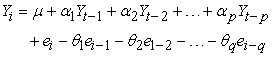
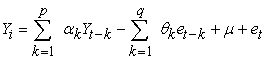
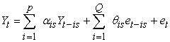
According to ^[7], autocorrelation patterns may require more complex models. A more General model is a mixture of the AR(p) and MA(q) models and is called autoregressive moving-average model, ARMA(p, q) model . He explained further that this model forecasts Y as both a linear combination of actual past values and a linear combination of past errors. The general ARMA (p, q) model is given by

(1)

(2)

Like the AR (p) model, the ARMA (p, q), has autocorrelation that diminish as the distance between residuals increases.

The order of the autoregressive component is p, the order of differencing needed to achieve stationarity is d, and the order of the moving average component is q. In general the ARIMA process (8) is of the form

(3)

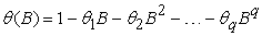
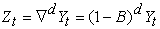
To express and understand differenced ARIMA models the concept of the backshift (lag) operator, B, and difference operator, ∇, is used, These has no mathematical meaning other than to facilitate the writing of different type of models that would otherwise be extremely difficult to express. The backshift is defined as . For example .

, and . The difference operator takes the form , when d differences are taken to achieve stationarity in the time series data. Using these notations,

1. The general AR(p) model 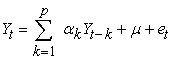is expressed as , where is the autoregressive operator of order p, defined by

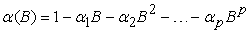(4)

2. The general MA (q) model 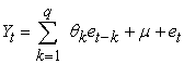is expressed as 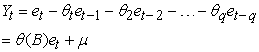where (B) is the moving average operator of order q, defined by

(5)

3. The general ARMA (p, q) model,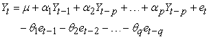, is expressed as

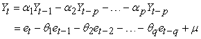
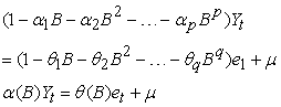(6)

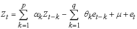
4. Stationary series obtained after d differencing of T is given by

(7)

5. A general ARIMA (p, d, q) model is expressed

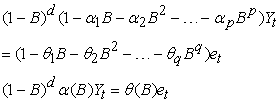(8)

Table 1. General Time Series Models

Download as

PowerPoint Slide

Larger image(png format)

Tables index

Veiw figure

View current table in a new window

View next table

Table 1 gives the summary of the general non seasonal time series models and their statistical properties. The table summarizes discussions on general AR, MA, and mixed ARMA ^[8] models.

A purely seasonal time series is the one that has only seasonal AR or MA parameters. Seasonal autoregressive models are built with parameter called seasonal autoregressive (SAR) parameters. The SAR parameters represent the autoregressive relationships that exist between time series data separated by multiples of the number of periods per season. A general AR model with P SAR parameters is given by 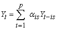where is of order s, is of order 2s and , is of order

ps. A model with one SAR parameter is written as

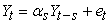(9)

Seasonal moving Average (SMA) models are built with seasonal moving average (SMA) parameters, and the general SMA model with Q parameters is given by:

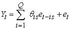(10)

The general mixed SAR and SMA model is given by

(11)

The order the seasonal ARMA process is given in terms of both Ps and Qs

Table 2 gives the summary of the stationarity and invertibility conditions of some specific seasonal time series models and the behaviour of their theoretical ACF and PACF.

Table 2. Specific Pure Seasonal Time Series Models

Download as

PowerPoint Slide

Larger image(png format)

Tables index

Veiw figure

View current table in a new window

View previous table

View next table

4. Data on Nigeria’s Inflation

Looking at Table 9 in the Appendix, it shows the data of ’s monthly inflation ratess from November 2003 to October 2013, totaling one hundred and twenty (120) monthly observations. The data were obtained from the National Bureau of Statistics. Figure 1 and Figure 2 show the plot of Nigeria’s monthly inflation and the trend analysis plot respectively. Figure 3 and Figure 4 also describe the features of the data that is the autocorrelation plot and the partial autocorrelation plot respectively.

Figure 1. TIME SERIES PLOT OF NIGERIAN’S MONTHLY INFLATION

Download as

PowerPoint Slide

Larger image(png format)

Figures index

Veiw figure

View current figure in a new window

View next figure

Figure 2. TREND ANALYSIS PLOT OF NIGERIAN’S MONTHLY INFLATION

Download as

PowerPoint Slide

Larger image(png format)

Figures index

Veiw figure

View current figure in a new window

View previous figure

View next figure

Figure 3. AUTOCORRELATION PLOT OF NIGERIA’S INFLATION

Download as

PowerPoint Slide

Larger image(png format)

Figures index

Veiw figure

View current figure in a new window

View previous figure

View next figure

Figure 4. PARTIAL AUTOCORRELATION PLOT OF NIGERIAN’S INFLATION

Download as

PowerPoint Slide

Larger image(png format)

Figures index

Veiw figure

View current figure in a new window

View previous figure

View next figure

Figure 5. ACF PLOT OF RESIDUALS OF NIGERIAN’S INFLATION

Download as

PowerPoint Slide

Larger image(png format)

Figures index

Veiw figure

View current figure in a new window

View previous figure

View next figure

A look at the time series plot of the original data in Figure 1 implies that the series is non-stationary. More so, the trend analysis as shown in Figure 2 shows a decreasing trend. However, the ACF plot as shown in Figure 3 dies down in a sinewave fashion and the PACF plot as shown in Figure 4 tails off at lag 2 (though there is a spike at lag 28, it is considered spurious and therefore neglected). With these results above, an AR ^[2] model is suspected. The result of estimates of parameters, the ACF and the PACF of the residuals obtained using MINITAB version 15.0 are shown below, Figure 5 and Figure 6 respectively.

Table 3. ESTIMATES OF PARAMETERS FOR AR(2) MODEL

Download as

PowerPoint Slide

Larger image(png format)

Tables index

Veiw figure

View current table in a new window

View previous table

View next table

Number of observations: 120

Residuals: SS = 393.856 (back forecasts excluded)

MS = 3.366 DF = 117

Figure 6. PACF PLOT OF RESIDUALS OF NIGERIAN’S INFLATION

Download as

PowerPoint Slide

Larger image(png format)

Figures index

Veiw figure

View current figure in a new window

View previous figure

View next figure

Figure 7. TIME SERIES PLOT FOR FORCAST USING AR (2)

Download as

PowerPoint Slide

Larger image(png format)

Figures index

Veiw figure

View current figure in a new window

View previous figure

View next figure

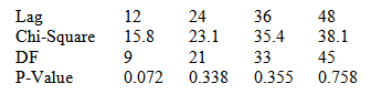
A look at Figure 6 and Figure 7 show some significant number of spikes outside the limit 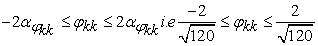which equals 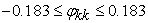suggesting that the residuals are not random. Figure 5 also shows that the P-values for the Ljung-Box statistics are significant. The forecast as shown by Figure 7 do not seem to be consistent with the forecast of inflation figures. We try differencing the data to bring about stationarity in mean.

Figure 8. TIME SERIES PLOT OF 1ST DIFFERENCE OF THE ORIGINAL DATA

Download as

PowerPoint Slide

Larger image(png format)

Figures index

Veiw figure

View current figure in a new window

View previous figure

View next figure

Figure 8 shows the time series plot of the first difference of Nigerian’s original inflation data. There is stationarity in mean and the existence of seasonality is evident.

Figure 9. TREND ANALYSIS FOR IST DIFFERENCE OF THE ORIGINAL DATA

Download as

PowerPoint Slide

Larger image(png format)

Figures index

Veiw figure

View current figure in a new window

View previous figure

View next figure

Figure 10 and Figure 11 show the autocorrelation function and the partial autocorrelation function of the first difference of Nigerian’s original inflation data respectively. The ACF and PACF show insignificant number of spikes dieing down in a sinewave fashion.

Figure 10. ACF OF IST DIFFERENCE OF THE ORIGINAL DATA

Download as

PowerPoint Slide

Larger image(png format)

Figures index

Veiw figure

View current figure in a new window

View previous figure

View next figure

Figure 11. PACF OF 1ST DIFFERENCE OF ORIGINAL DATA

Download as

PowerPoint Slide

Larger image(png format)

Figures index

Veiw figure

View current figure in a new window

View previous figure

View next figure

Figure 12. TIME SERIES PLOT OF THE SEASONAL DIFFERENCE OF THE 1ST DIFFERENCE DATA

Download as

PowerPoint Slide

Larger image(png format)

Figures index

Veiw figure

View current figure in a new window

View previous figure

View next figure

Figure 12 shows the time series plot of the seasonal difference of the first differenced of Nigerian’s inflation data which shows stability in mean at both the seasonal and the non-seasonal levels.

Figure 13. TREND ANALYSIS OF THE SEASONAL DIFFERENCE OF THE 1ST DIFFERENCED DATA

Download as

PowerPoint Slide

Larger image(png format)

Figures index

Veiw figure

View current figure in a new window

View previous figure

View next figure

Figure 13 shows the trend analysis of the seasonal difference of the first differenced of Nigerian’s original inflation data. The trend is neither increasing nor decreasing which is indicative of stationarity in mean.

Figure 14 shows the autocorrelation function of the seasonal difference of the first differenced of Nigerian’s original inflation data.

Figure 14. ACF OF THE SEASONAL DIFFERENCE OF THE 1ST DIFFERENCED DATA

Download as

PowerPoint Slide

Larger image(png format)

Figures index

Veiw figure

View current figure in a new window

View previous figure

View next figure

The time series plot of the 1st differenced data and the trend analysis as indicated in Figure 8 and Figure 9 show stationarity in mean and variance. There were significant spikes in the time series plot at lags 12, 24, and so on. This is indicating that seasonality is evident in the monthly inflation rates with a period of 12. This call for seasonal differencing of the 1st non-seasonal differenced data, as shown in Figure 12. Figure 10 and Figure 11 are the plots of the autocorrelation function (ACF) and the partial autocorrelation function (PACF) of the 1st differenced data. The ACF dies down after lag 1 and the PACF also tails off after lag 1, suggesting that p=1 and q=1 would be needed to describe these data as coming from a non-seasonal autoregressive and a moving average process respectively. Hence, the time series model that gives rise to these observations was an ARIMA (1, 1, 1) model, since the data was differenced once (i.e. d=1) to attain stationarity.

Figure 12 and Figure 13 show the time series plot of the seasonal difference of the 1st differenced series and the trend analysis plot respectively. The trend analysis shows stationarity at the seasonal level. Figure 14 and Figure 15 show the ACF and the PACF of the seasonal difference of the 1s differenced series respectively. A critical look at the seasonal lags show that both ACF and the PACF spikes at seasonal lag 12 dies down to zero for other seasonal lags, suggesting that p=1 and q=1 would be needed to describe these data as coming from a seasonal autoregressive and moving average process.

Figure 15. PACF OF THE SEASONAL DIFF. OF THE 1ST DIFFERENCED DATA

Download as

PowerPoint Slide

Larger image(png format)

Figures index

Veiw figure

View current figure in a new window

View previous figure

View next figure

Two goodness-of-fit statistics that are most commonly used for the model selection are; Akaike Information Criterion (AIC) and Schwarz Bayesian Information Criterion (BIC). The AIC and BIC are determined based on a likelihood function. The AIC ^[9] and BIC are calculated using the formulas below: and 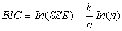where n is the total number of observations, SSE is the sum of the squared errors, and . In this paper, n = 120 data points. Four tentative ARIMA models are tested for the data series and the corresponding AIC and BIC values for the models are presented in Table 4.

Table 4. AIC and BIC values for four Tentative SARIMA Models

Download as

PowerPoint Slide

Larger image(png format)

Tables index

Veiw figure

View current table in a new window

View previous table

View next table

The models that have the lowest AIC and BIC are ARIMA (1 1 1) (0 0 1)¹² and (1 1 1) (1 0 1)¹² . Since two models are identified, the most suitable model is selected by the principle of parsimony. ARIMA (1 1 1) (0 0 1)¹² model has fewer parameters than ARIMA (1 1 1) (1 0 1)¹² model. Furthermore all the coefficients of ARIMA (1 1 1) (0 0 1)¹² model are significantly different from zero and the estimated values satisfy the stability as indicated in Table 3. We then proceed to the next stage of the Box-Jenkins approach which is the estimation of parameters of the tentative model.

Immediately a suitable SARIMA (P, d, q)(P, D,Q)¹² structure is identified, the next step is the parameter estimation or fitting stage. The parameters are estimated by the maximum likelihood method. The results of parameter estimations are reported in Table 5 and Table 6.

Table 5(a). Estimates of parameters of SARIMA (1, 1, 1) (1, 0, 1)¹² model

Download as

PowerPoint Slide

Larger image(png format)

Tables index

Veiw figure

View current table in a new window

View previous table

View next table

Differencing: 1 regular difference

Number of observations: Original series 120, after differencing 119

Residuals: SS = 227.986 (back forecasts excluded)

MS = 1.982 DF = 115

Table 5(b). Modified Box-Pierce (Ljung-Box) Chi-Square Statistic

Download as

PowerPoint Slide

Larger image(png format)

Tables index

Veiw figure

View current table in a new window

View previous table

View next table

Table 6(a). Estimates of parameters of the tentative SARIMA (1, 1, 1) (0, 0, 1)¹² model

Download as

PowerPoint Slide

Larger image(png format)

Tables index

Veiw figure

View current table in a new window

View previous table

View next table

Differencing: 1 regular difference

Number of observations: Original series 120, after differencing 119

Residuals: SS = 224.666 (back forecasts excluded)

MS = 1.937 DF = 116

Table 6(b). Modified Box-Pierce (Ljung-Box) Chi-Square Statistic

Download as

PowerPoint Slide

Larger image(png format)

Tables index

Veiw figure

View current table in a new window

View previous table

View next table

We proceed in our analysis to check if the parameters contained in the models are significant. This ensures that there are no extra parameters present in the model and the parameters used in the model have significant contribution, which can provide the best forecast. The estimates of autoregressive, moving average and the seasonal moving average parameters are labeled “AR..1”, “MA..1” and “SMA..12”, which are -0.6413, -0.8268, and 0.8840, respectively. Based on 95% confidence level, we conclude that all the coefficients of the ARIMA (1, 1, 1) (0, 0, 1)¹² model are significantly different from zero as shown in Table 3(a). Furthermore, the p-vales for the Ljung-Box statistic clearly all exceed 5% for all lag orders, implying that there is no significant departure from white noise for the residuals. We then proceed to the next step after parameter estimation which is the Diagnostic Checking or model validation. The Box and Jenkins (1970) estimation process for seasonal ARIMA model is shown in Figure 16.

The model verification is concerned with checking the residuals of the model to determine if the model contains any systematic pattern which can be removed to improve on the selected ARIMA model. It is obvious that the selected model may appear to be the best among a number of models considered; it becomes necessary to do diagnostic checking to verify that the model is adequate. Verification of an ARIMA model is tested (i) by verifying the ACF of the residuals, (ii) by verifying the normal probability plot of the residuals.

Figure 16. ACF of Residuals for SARIMA (1, 1, 1) (0, 0, 1)¹² model

Download as

PowerPoint Slide

Larger image(png format)

Figures index

Veiw figure

View current figure in a new window

View previous figure

Looking at Figure 16, the autocorrelation checks of the residuals indicate that the model is good because they a white noise process. That is the residuals have zero mean, constant variance and also uncorrelated. Also, the p-values for the Ljung-Box statistic from Table 3 as shown clearly exceed 5% for all lag orders, indicating that there is no significant departure from white noise for the residuals. Since the model diagnostic tests show that all the parameter estimates are significant and the residual series are random, it can then be concluded that (1, 1, 1) (0, 0, 1)¹² model is adequate for the inflation series. Therefore, (1, 1, 1) (0, 0, 1)¹² is used to forecast the inflation series of Nigeria.

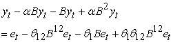
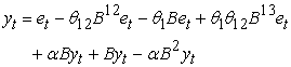
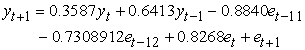
The ARIMA (1, 1, 1)(0, 0, 1) is selected to forecast the inflation variable, where autoregressive term p = 1(non-seasonal), P = 0(seasonal) [that is, (1 - αB)(1 – 0)]; differencing term d = 1(non-seasonal difference), Q = 0(seasonal difference) [that is (1 - B)(1 – 0)] and moving average term q = 1(non-seasonal), Q = 1(seasonal) [that is (1 - θ₁B)(1 - θ₁₂B¹²). For the dataset in Table 3, the fitted model is given by

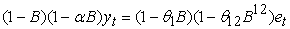(12)

(13)

Transforming the back operator, equation (13) becomes;

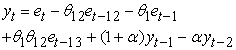(14)

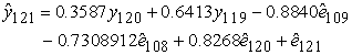
In order to forecast one period ahead that is, y_t+1, the subscript of the equation (14) is increased by one unit throughout as given by

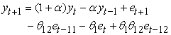(15)

The term e_t+1 is not known because the expected value of future random errors has been taken as zero. There are 120 data points from November 2003 to October 2013 used to build the ARIMA model. From the Table 3, using α = -0.6413, θ₁ = -0.8268, θ₁₂ = 0.8840, we have θ₁θ₁₂ = -0.7308912. Thus, equation (15) is given as

In order to forecast inflation for the period 121 (that is, November 2013), equation (15) is given by

The forecast quantity for period 121 can now be calculated as follows:

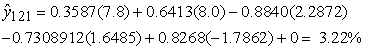Once our model has been obtained and its parameters have been estimated, we can use it to make our prediction. Table 7 summarizes 12 months upfront inflation forecast from November 2013 to October 2014 with 95% confidence interval.

Table 7. 12- Month Forecasted Inflation for November 2013 to October 2014

Download as

PowerPoint Slide

Larger image(png format)

Tables index

Veiw figure

View current table in a new window

View previous table

View next table

Table 8. Basic Statistic of Nigeria’s Monthly Inflation Data in Percentages

Download as

PowerPoint Slide

Larger image(png format)

Tables index

Veiw figure

View current table in a new window

View previous table

View next table

5. Conclusion

From Figure 1, it can be confirmed that inflation exhibit volatility starting from somewhere around 2006. The volatility in Nigerian’s inflation series can be attributed to several economic factors. Some of these factors are money supply, exchange rates depreciation, petroleum price increases, and poor agricultural production.

Box-Jenkins Seasonal Autoregressive Integrated Moving Average (SARIMA) was employed to analyze monthly inflation rates of Nigeria from October 2003 to November 2013. The study mainly intended to forecast the monthly inflation rates for the coming period of November, 2013 to November 2014.

Series of tentative models were developed to forecast Nigeria’s monthly inflation, but based on minimum AIC and BIC values and after the estimation of parameters and series of diagnostic test were performed, ARIMA(1,1,1)(0,0,1) 12 model was judge to be the best model for forecasting after satisfying all model assumptions.

The forecast results revealed a decreasing pattern of inflation rates in the first quarter of 2014 and turning point at the beginning of the second quarter of 2014, where the rates takes an increasing trend till the September.

Definition of Terms

The full meanings of the abbreviations used in this paper are:

ACF – Autocorrelation function

PACF – Partial Autocorrelation function

AR – Autoregressive

MA – Moving Average

SMA – Seasonal Moving Average

SAR – Seasonal Autoregressive

ARIMA – Autoregressive Integrated Moving Average

SARIMA – Seasonal Autoregressive Integrated Moving Average

AIC – Akaike Information Criterion

BIC – Bayesian Information Criterion

APPENDIX-A

Table 9. Nigeria’s Monthly Inflation Ratess from November 2003 to October 2013

Download as

PowerPoint Slide

Larger image(png format)

Tables index

Veiw figure

View current table in a new window

View previous table

References

[1]	Rudiger Dornbusch and Stanley Fischer, (1993). “Moderates Inflation”, The Bank Economic Review, Vol.7, Issue 1, Pp.1-44.
	In article		CrossRef
[2]	Jack H.R, Bond M.T., and Webb J.R, (1989). “The Inflation- Hedging Effectiveness of Real Estate”. Journal of Real Estate Research, Vol.4. Pp. 45-56.
	In article
[3]	Hamidreza M. and Leila S. (2012). Using SARFIMA model to study and predict the Iran’s oil supply. International Journal of Energy Economics and Policy. Vol.2, No.1, 2012, pp.41-49.
	In article
[4]	Fritzer, F., Gabriel, M. and Johann, S. (2002). "Forecasting Austrian HICP and its Components using VAR and ARIMA Models," Working Papers 73, Oesterreichische National bank (Austrian Central Bank).
	In article
[5]	Gomez V., and Maravall A., (1998.) "Automatic Modelling Methods for Univariate Series," Banco de España Working Papers 9808, Banco de España.
	In article
[6]	Leila S. and Masoud Y. (2012). An Empirical Study of the Usefulness of SARFIMA models in Energy Science. International Journal of Energy Science. IJES Vol.2 No.2 2012.
	In article
[7]	[Jeffrey J., (1990). “Business forecasting Methods”. Atlantic Publishers.
	In article
[8]	Box, G. E. P and Jenkins, G.M., (1976). “Time series analysis: „Forecasting and control,” Holden-Day, San Francisco.
	In article
[9]	Akaike, H. (1974). A New Look at the Statistical Model Identification. IEEE Transactions on Automatic Control 19 (6): 716-723.
	In article		CrossRef