1. Introduction

During the last century, splines theory has received considerable attention. Lacunary interpolation was initiated in 1957 ^[1]. Several researchers have studied the use of splines to solve such interpolation problems ^{[2, 3, 4, 5]}. All of these methods are global and require the solution of a large system of equations. The most appropriate method solving lacunary interpolation problems using piecewise polynomials with certain continuity properties.

Spline functions are a good tool for the numerical approximation of functions on the one hand and they also suggest new, challenging and rewarding problems on the other. Piecewise linear functions, as well as step functions, have been an important theoretical and practical tools for approximation of such functions. Lacunary interpolation by spline appears whenever observation gives scattered or irregular information about a function and it's derivatives. Also, the data in the problem of lacunary interpolation are values of the functions and of it's derivatives but without hermite condition in which consecutive derivatives are used at each nodes.

2. Construction

Let S(x) ε S⁽⁵⁾_n,6 denote the class of sixtic splines S(x) on [0,1] such that

•  S(x) ε C⁵ [0, 1]

•  S(x) is a polynomial of degree six on each subinterval

(1)

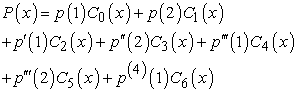
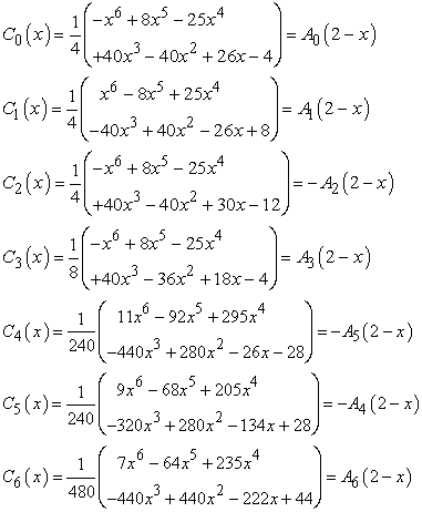
It can be verified that if P(x) is a sixtic on [0, 1] then:

Where:

(2)

For later references we have:

and

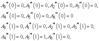and

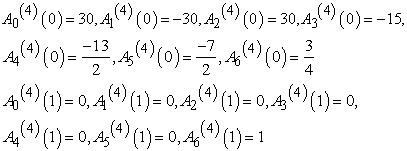and

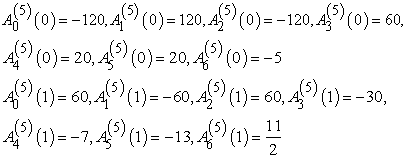Further, a sixtic P(x) on [1, 2] can be written as:

Where:

(3)

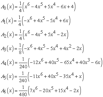
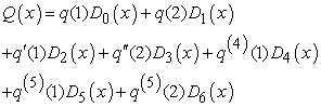
It is easy to verify that a sixtic Q(x) on [0, 1] can be expressed in the following form:

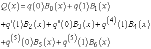(4)

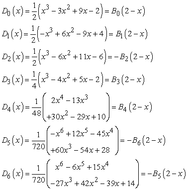
Where:

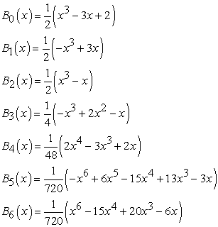(5)

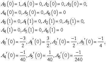
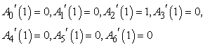
for later references we have

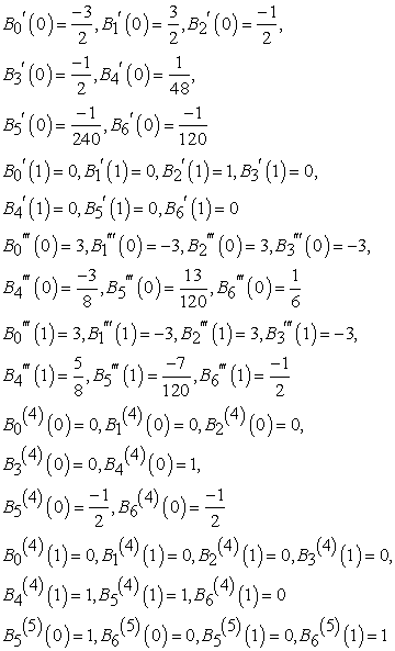Also a sixtic Q(x) on [1, 2] can be written as:

(6)

Where:

(7)

3. The Approximation of the Spline Functions

Descriptions of the method: Let (S_n, C⁵) be the class of spline functions with respect to the set of knots x_i. The spline functions will denoted by S_i(x), where i = 0, 1,..., n. We shall prove the following:

Theorem 1 (Existence and Uniqueness)

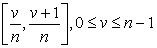
For every odd integer n and for every set of 5n+9/2 real numbers

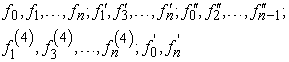there exists a unique S(x) ε S⁽⁵⁾_n,6 such that:

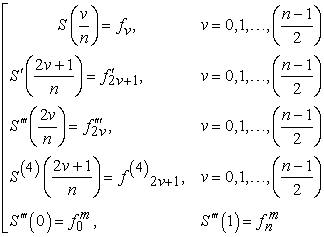Let fεC⁵[0,1] and n an odd integer. then the unique sixtic spline S_n(x) satisfying conditions of Theorem 3.1, with f_v = f(v/n), v = 0,1,…,n;

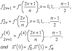(8)

we have:

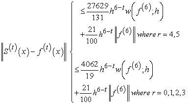Proof of Theorem 1

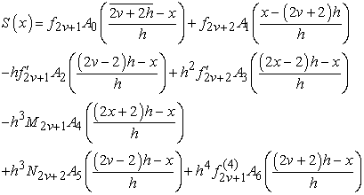
For a given S(x) ε S⁽⁵⁾_n,6 set h = n^-1, M_v = S⁽⁵⁾ (vh+), v = 0,1,…..,n-1, Nv = S⁽⁵⁾ (vh-), v = 0,1,….,n. Since, S⁽⁵⁾ is linear in each internal (vh, (v+1)h), it is completely determined by the (2n) constants 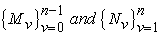. Also, if S(x) satisfies the requirements of Theorem 1 that for 2vh ≤ x ≤ (2v+1)h, v = 0,1,…, n-1/2 , it must have the following form:

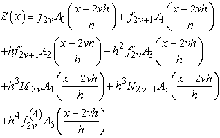(9)

and for (2v+1)h ≤ x ≤ (2v+2)h , v=0,1,…., n-3/2, S(x) has the form:

(10)

We shall show that it is possible to determine the (2n) parameters , such that the function S(x) given by Eq. 9 and 10 will also satisfy (5) in Theorem 1 and S' (x), S"(x) and S⁽⁴⁾ will be continuous on [0,1]. S(x) is continuous because of the interpolating condition Eq. 8 in Theorem 1, S'(x) and S⁽⁴⁾(x) are continuous on [0,1] except at the points (2vh) and (2v+1)h, respectively, v = 0, 1,… , n-1/2.

From Eq. 10 we see that Eq. 8 in Theorem 1 is equivalent to:

(11)

(12)

Simple calculations show that S"((2v+2)h-) = S"((2v+2)h+) and S⁽⁵⁾((2v+2)h+) are equivalent to:

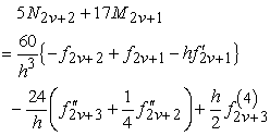(13)

(14)

Similarly 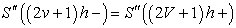and 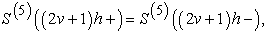are equivalent to:

(15)

(16)

Thus, the theorem will be established if we show that the system of linear Eq. 12-16 has a unique solution. This end will be achieved by showing that the homogeneous system corresponding to Eq. 12-16 has only zero solution.

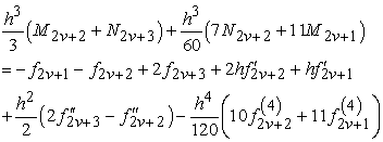
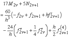
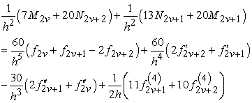
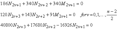
The following is the homogeneous system of equations for v= 0,1,…, n-3/2:

(17)

(18)

(19)

(20)

(21)

(22)

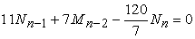
Form Eq. 19 and 20 we have for v = 0, 1,…, n-3/2:

and

(23)

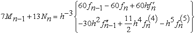
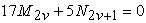
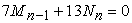
Putting the values and M_n-1 = -13/7 N_n from Eq. 19 in 20 we have:

(24)

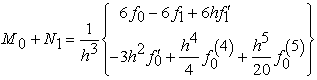
Also, from Eq. 14 and 20 we have:

(25)

and M₀ = -N₁ from Eq. 21.

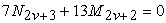
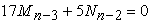
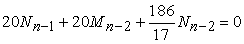
Using Eq. 19 we obtain 17M_n-3+5N_n-2 and using Eq. 21 with 25 and 24 we have M_n-3 = N_n-2 = M_n-2 = N_n-1 = 0. Also obtain the system:

By the same manner we get M₀ = M₁ = … = M_n-1 = 0 and N₁=N₂= N₃ = … = N_n = 0, to solution of the homogeneous system for n = 4p and n = 4p+2.

References

[1]	J. BALAZS AND P. TURAN, Notes on interpolation. II, III, IV, Acta Math. Acud. Sci.Hungar, 8 (1957), 201-215; 9 (1958), 195-214, 243-258.
	In article
[2]	TH. FAWZY, Note on lacunary interpolation with splines. 1. (0, 3)-Lacunary interpolation,Ann. Univ. Sci. Budapest. Eiifciis Sect. Math. 28 (1985).
	In article
[3]	TH. FAWZY, Note on lacunary interpolation by splines. II, Ann. Univ. Sci. Budapest. Sect.Comput. 5, in press.
	In article
[4]	TH. FAWZY, Notes on lacunary interpolation by splines. III. (0, 2) Case, Acra Math. Acud.Sci. Hungar., in press.
	In article
[5]	TH. FAWZY, Lacunary interpolation by g-splines: (0, 2, 3) Case, Studia Sci. Math.Hungar., in press.
	In article